")
")
| Issue |
Int. J. Simul. Multidisci. Des. Optim.
Volume 8, 2017
|
|
|---|---|---|
| Article Number | A7 | |
| Number of page(s) | 10 | |
| DOI | https://doi.org/10.1051/smdo/2016016 | |
| Published online | 23 January 2017 | |
Research Article
An assembly oriented design and optimization approach for mechatronic system engineering
1
ICB UMR 6303, CNRS, Univ. Bourgogne Franche-Comté, UTBM, 90010
Belfort, France
2
ERPI, Université de Lorraine, 54510
Nancy, France
* e-mail: This email address is being protected from spambots. You need JavaScript enabled to view it.
Received:
21
October
2016
Accepted:
22
November
2016
Abstract
Today, companies involved in product development in the “Industry 4.0” era, need to manage all the necessary information required in the product entire lifecycle, in order to optimize as much as possible the product-process integration. In this paper, a Product Lifecycle Management (PLM) approach is proposed, in order to facilitate product-process information exchange, by considering design constraints and rules coming from DFMA (Design For Manufacturing and Assembly) guidelines. Indeed, anticipating these manufacturing and assembly constraints in product design process, reduces both costs and Time To Market (TTM), and avoids to repeat mistakes. The paper details the application of multi-objective optimization algorithms after considering DFMA constraints in a PLM approach. A case study using an original mechatronic system concept is presented, and improved by considering product-process integrated design, optimization and simulation loops, using numerical optimization and FEM (Finite Element Method) methods and tools.
Key words: Product lifecycle management / Design for manufacturing and assembly / Multi-objective optimization / Finite element modeling and simulation
© B. Marconnet et al., published by EDP Sciences, 2017
 This is an Open Access article distributed under the terms of the Creative Commons Attribution License (http://creativecommons.org/licenses/by/4.0), which permits unrestricted use, distribution, and reproduction in any medium, provided the original work is properly cited.
Symbols
α : Battery maximum discharge
C : Battery capacity
D : Propeller diameter
F : Drone weight
h : Propellers geometrical pitch
M : Total mass – drone
p : Air pressure
ρ : Air density
S : Circular area used by the propellers
Δt : Autonomy (flight time)
T : Thrust
T b : Battery voltage
v : Speed induced by the propeller
V : Air speed
ω : Engine revolution
W st : Power needed to maintain the stationary position during flight
1 Introduction
Over the last two decades, the industrial context has lead companies to be more and more competitive, especially in their engineering processes. As such, the use of formalized design approach combined with optimization methods, plays an important role in the product-process design lifecycle. This challenge will enable designers and engineers to be assisted in their design activities with the support of models, methods and tools covering the whole product lifecycle [1]. Although some interesting research results have been successfully applied in industry, some design mistakes remains due to interoperability barriers in information systems covering design, engineering and manufacturing phases [2]. Exploiting a product lifecycle management (PLM) approach with collaborative design tools [3], allows to manage all the required information and knowledge of a product in its entire lifecycle (from the emergence of its concept until its recycling). Moreover, the decision-making in product design requires to estimate, at best, all lifecycle process constraints, in the appropriate context. For the need of our research work, we exploited the PLM approach and optimization methods through the development process of optimized products [4] in order to do new design iteration loops of a concept, based on assembly and manufacturing analysis. The aim of our project, is to apply our design principles to an innovative concept of a “Follow Me” drone, as an answer to the following needs, inspired from the Nixie project1: record, assist and follow its owner, with the possibility to be attached at his wrist as a connected watch. Nowadays, more and more people, practicing outdoor physical activities, need a portable video system (e.g. camera, drone) which have the functionality to record videos and diffuse important information from “difficult to reach” locations. These kind of devices allow the user to record and control manually or automatically these system, for “extreme activities” (sport, security, defence, etc.). Another use of these kind of drones, is to help users to make various points of view (e.g. Selfie) in an autonomous manner. It exist some products which are able to follow and film their owner (like “Follow Me Drones” or “Flying selfie Bots” [5]). Besides this need, people are now more and more connected, thanks to connected watches (e.g. Samsung Galaxy Gear), they are now able to read, manage and follow their activities in order to improve their skills every day. By anticipation of the future evolution of these kinds of concept, we decide to design such a product, by following our own PLM approach integrating parametric CAD modeling and optimization loops. The development of this kind of product, allows us to manage in a better manner, the product information all along its design lifecycle. Two modeling and optimization methods have been applied in the product design process in order to find a generic formulation. The first method is the multi-objective optimization (activated in order to find the best solution) and the second is the exploitation of Finite Element Method, applied in order to predict the product behavior under specific multi-physics loads.
2 Toward a skeleton definition approach to the multi-objective optimization principles
The most important elements in the PLM approach, are the steps that link each part to the others, thanks to collaborative platforms. We use a method for designing and modeling products in a top-down design process, named SKL-ACD (SKeLeton-based Assembly Context Definition) [6, 7]. Based on kinematic and technology pairs definition, at the early stages of the design process, the SKL-ACD approach generates the product’s skeleton geometry (i.e. points, lines, planes, etc.) in a CAD (Computer Aided Design) environment, skeleton parameters and the required constraints between the skeleton entities. From this skeleton point of view, functional surfaces and design spaces are developed. The detail design is then obtained, by choosing the best technical solution based on constraints and behavior objectives. Thus, the product optimization loop can be applied by using multi-objective optimization algorithms, in order to select the best available options, from a wide range of possible choices [8]. A single-objective optimization approach is not sufficient to deal with real-life problems. In fact, engineers are frequently asked to solve problems with several conflicting objective functions. Multi-disciplinary and multi-objective optimization consists in finding the optimal design of complex engineering systems which requires analysis that takes into account interactions among the disciplines (or parts of the system) and which seeks to synergistically exploit these interactions. Figure 1 introduces our product design process, with the SKL-ACD approach, in order to develop and optimize the product.
 |
Figure 1. Design steps with the SKL-ACD approach. |
Step 1: The first step of the project is to specify all the requirements and functions and to derive a final concept based on this information. It was important to define information about requirements, objective functions, constraints, and rules used for the optimization steps.
Step 2: It starts with the list of all the components of the designed product, and then to apply relationships between each of these components in order to create the directed graph. This graph leads to an adjacency matrix, which will be used to define sub-assemblies. Sub-assemblies are divided in three categories: serial, parallel or interconnected. To define these assemblies, it is possible either to make some matrix calculations, or more simply to use a dedicated software, which automatically generates admissible assembly sequences, by a simple drawing of the directed graph on the software. The selected assembly sequence will lead to the mBOM (manufacturing Bill Of Material), which is a structured copy of the eBOM (engineering Bill Of Material). Because the latter just lists all the components of the product, instead to the mBOM, which shows, by structural means, the relationships between each component and particularly the final structure of the product. Besides, this mBOM is the basis of the main part of the process: the skeleton.
Steps 3–8: The direct graph leads to the skeleton elements (plane, line, curves, points, etc.) based on assembly constraints, which will be then linked and structured together, in order to form a skeleton minimal graph. This simplified graph represents all the necessary elements of the skeleton, which will be used for assembling all the parts of the products. Only then, using the mBOM and the skeleton minimal graph, it will be possible to construct the skeleton on CAD and add the product with all its components. Thanks to this approach, when an element of the product is moved, only one of the skeleton elements is to be changed, and all the assembly will update accordingly.
Step 9: After all these steps of design, come two last steps which will consist in analysing and optimizing the designed product in order to shorten the development time, the assembly time, and also to reduce cost of production by correcting the design errors. DFMA analysis [9] help designers, to evaluate the assembly/manufacturing mistakes, on the product geometry, by searching through a guideline, all process constraints. To go on, we will use the DFA (Design For Assembly) and DFM (Design For Manufacturing) analysis, which are tools used to optimize the quoted criteria before. In the DFA analysis, assembly efficiency of a product is evaluated, by using a metrics called the design efficiency: where:
-
t a: Basic assembly time, it’s the average time for a part that presents no handling, insertion, or fastening difficulties (about 3 s).
-
N min: Theoritical minimum number of parts.
-
T total: Estimated time to complete the assembly of the product represented by: Instance number of the component in the product × (Manual handling time (s) + Manual insertion time (s)).
According of the DFMA analysis, if efficiency is more that 60%, a product will be considered as ease for assembly if E > 60%. Otherwise a redesign of the product will be needed. Based on the result of the DFMA analysis, we apply the optimization methods. From a mathematical point of view, a multi-objective optimization problem can be written as follows:![Mathematical equation: $$ \begin{array}{c}\mathrm{min}[{f}_1(X),{f}_2(X),\dots,{f}_i(X)],\\ {G}_j(X)\ge 0,\mathrm{and}\enspace {G}_1(X)=0,\\ X=({x}_1,\dots,{x}_{n+u})\end{array} $$](/articles/smdo/full_html/2017/01/smdo160012/smdo160012-eq2.gif) where:
where:
-
f 1 …, f i : objective functions, for the response parameters. When i > 1 and the different and conflicting functional requirements are observed, it is a multi-objective optimization problem. These are the quantities that the designer wishes to maximize or minimize.
-
G j (x 1, …, x n+u ) ≥ 0, and G 1(x 1, …, x n+u ) = 0: constraints. Equality and inequality constraints are imposed on the product design, directly connected to the requirements. These constraints correspond to the limits that the designer must meet due to the need to comply with standards, or due to the particular characteristics of the environment, functionalities, physical limitations, etc.
-
X = (x 1, …, x n+u ): vector of variable integrating generally the “n” customers’ requirements and “u” technical design parameters of the product. These variables are considered as input data of the optimization problem.
Step 10: The last step of the PLM approach will be to add the product on the PLM platform, which will manage the CAD assembly and all the information linked to the product. Thanks to the MPM, it will also be used to create an assembly range or a manufacturing range.
3 Experimental design case study
The product design begins by the study of the functional specification. The system would be able to follow and film the user, it has to be worn as a connected watch and must avoid obstacles; all these functions are to be fulfilled with a sufficient autonomy (min. 10 min). The concept shown in Figure 2 has been used to illustrate the proposed approach. This figure shows in the central part, the main body separated in four branches, which deploy under the magnetic effect of magnets. The most innovative part of the concept lies in this aspect, because when the magnets lift off, and motors start, the branches will deploy in the horizontal plane thanks to the force developed by the propellers. After this design step, we have defined all the elements of the drone, and thus realized the following eBOM.
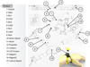 |
Figure 2. First design concept and its related eBOM. |
Owing the product’s symmetry, the eBOM has been realized for only a quarter of the product. eBOM was used to define the directed graph (Figure 3) which will be one of the bases of the skeleton. This last will generate the mBOM and the skeleton minimal graph.
 |
Figure 3. Definition of the direct graph. |
Based on this graph, we use the Pegasus software [6], in order to generate a list of possible assembly sequences (Figure 4), which need to be sorted in order to find the most suitable for our product. Algorithm ASDA (Assembly Sequence Definition Algorithm) exploit precedence constraints of product, in order to suggest, some possibility of this product to be assembled. It considers sub-assembly, base, assembly layer, assembly order of each parts in product.
 |
Figure 4 Generation of admissible assembly sequences. |
The following assembly sequence was selected, based on manufacturing context (Design Takt Time; Overall Equipment Effectiveness [OEE]). Expert process, and assembly planner choose one of this solution, in order to match with manufacturing objective:![Mathematical equation: $$ \{[(1,\enspace 13,\enspace 14,\enspace 17),\enspace 2],\enspace [6,\enspace (4,\enspace 3,\enspace 5),\enspace (8,\enspace 7,\enspace 9)],\enspace (10,\enspace 11,\enspace 15,\enspace 16),\enspace 12\} $$](/articles/smdo/full_html/2017/01/smdo160012/smdo160012-eq3.gif)
Final result has been checked in order to evaluate if this sequence truly corresponds to our product, while making manually the necessary matrix calculations (adjacency matrix, companion matrices, etc.). Now, as the mBOM was defined thanks to this sequence, the directed graph was used, in order to generate the skeleton minimal graph which will help to draw the skeleton on a CAD application: CATIA V5. To achieve this goal, first of all the links between each component are converted into assembly constraints, due to the fact that these assembly constraints are associated to geometrical elements. Using the SKL-ACD approach these assembly constraints are then replaced by their associated geometric elements which are subsequently linked considering specific geometrical relations (perpendicular, parallel, distance, etc.); this lead to the graph displayed in Figure 5. Only after these steps, we could generate the following skeleton minimal graph, which is a simplified version of the last graph.
 |
Figure 5. Steps from direct graph to skeleton minimal graph. |
With all the elements of the skeleton previously defined, the design can be moved to the next steps of the PLM approach: drawing the skeleton on Catia, based on the skeleton minimal graph. From the mBOM and the skeleton minimal graph, the skeleton of the product is generated, the product’s parts are then designed in detail on this basis (Figure 6).
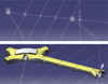 |
Figure 6. Skeleton and the first iteration in a CAD environment. |
At this stage, the skeleton is simplified because when we want to move a part or change the assembly, we just have to change the skeleton parameters. The first iteration of the concept shows the different parts which are placed on the different skeleton elements: for example, links and pins are placed on their axes and limited by one plane. After this process of design, DFA and DFM analyses were applied to the product, which will check and evaluate the parts individually using assembly/manufacturing rules.
The DFA analysis (Figure 7), shows that the product is pretty reliable about its assembly, but the product structure may be simplified by either reducing the number of pins (given the number important of these parts) or by consolidating the basis with the hull, which is therefore less possible. For the concept, the design efficiency is estimate to 37.4%.
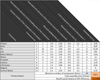 |
Figure 7. DFA analysis example. |
These analysis lead to the conclusion that the first iteration is not efficient for assembly (because the 60% limit is not reached); in addition, some errors were detected for manufacturing. An evolution of this concept, is required in order to redesign and change part/process type. For the proposition of the ideal product, an application of three rules, is called:
-
During the normal operating mode of the product, the part moves relative to all other parts already assembled. (Small motions do not qualify when they can be obtained through the use of elastic hinges.).
-
The part must be of a different material, or be isolated from all other parts assembled (for insulation, electrical isolation, vibration damping, etc.).
-
The part must be separate from all other assembled parts; otherwise, the assembly of parts meeting one of the preceding criteria would be prevented.
The DFM analysis, are used with the DFMPro software. This aim is to analyze the geometry of a specific part, and check all consistency rules. For example, a rule analyze, the draft angle of the cavity, and recommended a defined degrees.
After identify essential parts, we apply the PLM approach with an updated eBOM. The new DFA efficiency are estimate to 57.1%, and DFM analysis allow to see all rules based on process, which are respected in order to exploit multi-optimization. The project requirements were the base to the drone’s optimization. Requirements that will be used as constant or as minimum/maximum values during simulations are shown in Table 1.
Example of requirements for the optimal design.
Figure 8 presents a diagram that shows the principal relations between the main parts and parameters to evaluate the flight time. Motor, propeller and battery are the parts that may be changed according the performance and flight time wanted.
 |
Figure 8. Simplified diagram of relations between the main components or parameters in the optimization of the flight time. |
The parameters available to the simulation are shown in Table 2. The dimensions will change according to the presented limits. Epoxy resin will be used in most simulations. Even being a more expensive material, when compared to the ABS, the project requires god precision during 3D printing, what is possible just with the machines that works with resin. We exploit the simulated annealing algorithm (based on an analogy with the solidification of a fluid), because we need to achieve a faster solution indicating a low number of consecutive updates without improvements, this global stochastic search algorithm, so two successive executions of this method can give two different results. Performing a global search algorithm which operates, after a lapse of time, to local searches. Generally used in the case of functions (objectives and constraints) non-linear, these functions may also be discontinuous.
Example of technical parameters.
The relations that connects the parameters with the results required, such as the constraints, are shown in Table 3. In order to complete requirements, technical parameters have added, by defining the continuous and discrete variables. For example, the description of the flight time, allows to find the best solution in the choice of the battery capacity.
Example of objective functions and constraints (variables description are detailed at the end of paper).
The rules used to evaluate the results are detailed in the Table 4. The first rule, for example, is used to verify if the thrust generated by the propellers is bigger than the thrust needed by the drone. The second rule verify the power generate by the propeller as being bigger than the power needed by the drone.
Example of rules used to verify the optimization criteria.
Considering the drone’s weight from the simulations and engines with a thrust superior to the total drone’s weight, several batteries with their respective prices, were used in order to compare three parameters: flight time, drone’s weight and battery capacity. The results, generated are shown in Figure 9.
 |
Figure 9. Optimization results between flight time, drone’s weight, price and battery capacity. |
It is important to say that the same battery capacity may have different flight times. It happens because the batteries may have different values of maximum discharge, factor that is also considered in the equation, and also leads to different battery weights. The optimal solution chosen is the battery with a capacity of 380 mAh. One of the choices is the requirement that must correspond to the minimum autonomy time. The price of the battery was the last decisive choice.
Once the solution has been chosen, the mechanical structure needs to be designed in order to resist falls and mechanical shocks. The critical case studied corresponds to a fall of 2 m until the ground, shown in Figure 10.
 |
Figure 10. Optimization based on a critical case – fall of 2 m absorbed by only one leg. |
The force equivalent to this fall was calculated considering that the kinetical energy is equal to a work with deformation of 0.5 mm. It resulted in an important force, using as reference the arm axis as x. To simulate this problem, a part was created considering two symmetries. The geometry reproduced one arm, attached to 1/4 of the electronic box.
The parameters shows in Table 5 were created and attributed to its respective dimensions in the geometry. In this way each dimension may vary freely between its limits.
Parameter and its limits used during the optimization in Catia.
The maximum displacement in the arm is of 10.8 mm, what represents 10% of the total arm length, which is almost 100 mm. Medium constraints reaches 60% of the material limit. There are a few points that presents elevated constraints, above the material tensile strength. A configuration with the minimum dimensions of all parameters (configuration A) is above the limit of mechanical resistance according to the project requirements. Configuration B presents a maximum displacement of 5.326 mm, a half of the displacement in the configuration A. The constraints are also smaller than in configuration A, but they are still in the limit of the material tensile strength. The small regions that presents the higher constraints may be also be generated by bad conditions in the mesh in these regions. A chamfer may help to decrease the maximum constraints. The same simulation was done with a different material, ABS (configuration D). However, it did not present considerable differences. Results may be seen in the Table 6.
Results of five simulations in different configurations.
The first simulation was done considering the material Epoxy Resin. The configuration A, with minimum values were used. Several parameters of five configurations which were simulated, are detailed. Configurations A, B and C have the same material in its composition. Configuration A presents the lowest parameters, and configuration B presents the highest ones. Configurations D and E are equals to A and B respectively, but are made of ABS. Configuration C has parameters with intermediary values. The ABS presents a bigger maximum displacement when compared to the Epoxy Resin. ABS parts are lighter than the others, but the biggest difference is the cost of the product. The heaviest configuration with ABS weights 79.99 g and costs 28 cents (the drone structure complete). On the other hand, the lightest part in epoxy resin weights 40.98 g and costs €12.29. The heaviest one costs €21. Configurations A, B and C are represented in the Figure 11. It is possible to see the difference in the parts width and thickness.
 |
Figure 11. Visualization of configurations A, B and C. |
4 Conclusion and future work
This PLM approach combined with optimization methods, allow to see the potential gain of the method in our case study. If the process is pretty long to generate the skeleton, we had seen that it has a very most important advantage compared to other methods. Particularly for assembly with many components. The analysis of a drone flight time was studied in details. Starting from fluid mechanics until reach electric power, in order to establish trustable relations between the main drone’s characteristics. All relations were developed, in order to estimate the drone’s autonomy. It was show that the relations present reasonable results, especially when considering the simplicity of the proposed relations. A mechanical analysis was done, evaluating the behavior of one arm of the drone when a force equivalent to a 2 m fall is applied. The model used is in the limit of the rupture. The effect of a geometry changing was shown in the analysis. A more detailed redesign must be done. An evolution of the prototype is necessary, in order implement the LCD screen, and increase the capacity of battery. Experimental tests with the prototype may provide data to verify the calculations and simulations done in this article.
Future work will consist of developing a HUB (The HUB is a central device that connects multiple computers on a single network2) which consists of designing in a PLM system, a model of collaborative platform, centralization and management information flows. The reasoning consists in developing an ontology, in order to make the logical inference in the HUB. Another vision can be given, with the application on the manufacturing aspects, for example once the design oriented assembly is completed. The designer can switch in the manufacturing context in order to detail and optimize the product, with appropriate knowledge.
Acknowledgments
The author would like to thank Dr. Nadhir Lebaal (associate professor at ICB laboratory) for his valuable assistance in the formulation of the optimization issue and ACCELINN company for this collaboration and all financial supports, under the supervision of James Garnier (PhD and Product-Process responsible from ACCELINN company) for his advice. Ana Bonato da Cruz (engineer student) for his help in the search for mechanical optimisation. This research work is made in collaboration with IRTES-M3M lab, as part of a CIFRE contract (Industrial Standards of Research Training) by the French National Agency for Research and Technology (ANRT).
References
- Liu W, Maletz M, Zeng Y, Brisson D. 2009. Product lifecycle management: a review. IDETC/CIE. ASME: San Diego, USA. [Google Scholar]
- Gregory T, Brunnermeier SB, Martin SA. 1999. Interoperability Cost Analysis of the U.S. Automotive Supply Chain. National Institute of Standards and Technology, Research Triangle Institute, Center for Economics Research, Final report RTI Project Number 7007-03. [Google Scholar]
- Kvan T. 2000. Collaborative design: what is it? Autom. Constr., 9(4), 409–415. [CrossRef] [Google Scholar]
- Eggers J, Feillet D, Kehl S, Oliver Wagner M, Yannou B. 2003. Optimization of the keyboard arrangement problem using an Ant Colony algorithm. Eur. J. Oper. Res., 148(3), 672–686. [CrossRef] [MathSciNet] [Google Scholar]
- Schneider D. 2015. Flying selfie bots. IEEE Spectrum, 52(1), 49–51. [CrossRef] [MathSciNet] [Google Scholar]
- Demoly F, Yan X-T, Eynard B, Rivest L, Gomes S. 2011. An assembly oriented design framework for product structure engineering and assembly sequence planning. Robot. Comput.-Integr. Manuf., 27(1), 33–46. [CrossRef] [Google Scholar]
- Demoly F, Toussaint L, Eynard B, Kiritsis D, Gomes S. 2011. Geometric skeleton computation enabling concurrent product engineering and assembly sequence planning. Comput. Aided Des., 43(12), 1654–1673. [CrossRef] [Google Scholar]
- Gomes S, Varret A, Bluntzer JB, Sagot JC. 2009. Functional design and optimisation of parametric CAD models in a knowledge-based PLM environment. Int. J. Prod. Dev., 9(1–3), 60. [CrossRef] [Google Scholar]
- Boothroyd G, Dewhurst P, Knight WA. 1994. Product design for manufacture and assembly. Comput. Aided Des., 26(7), 505–520. [CrossRef] [Google Scholar]
Cite this article as: Marconnet B, Demoly F, Monticolo D & Gomes S: An assembly oriented design and optimization approach for mechatronic system engineering. Int. J. Simul. Multisci. Des. Optim., 2017, 8, A7.
All Tables
Example of objective functions and constraints (variables description are detailed at the end of paper).
All Figures
|
Figure 1. Design steps with the SKL-ACD approach. |
| In the text | |
|
Figure 2. First design concept and its related eBOM. |
| In the text | |
|
Figure 3. Definition of the direct graph. |
| In the text | |
|
Figure 4 Generation of admissible assembly sequences. |
| In the text | |
|
Figure 5. Steps from direct graph to skeleton minimal graph. |
| In the text | |
|
Figure 6. Skeleton and the first iteration in a CAD environment. |
| In the text | |
|
Figure 7. DFA analysis example. |
| In the text | |
|
Figure 8. Simplified diagram of relations between the main components or parameters in the optimization of the flight time. |
| In the text | |
|
Figure 9. Optimization results between flight time, drone’s weight, price and battery capacity. |
| In the text | |
|
Figure 10. Optimization based on a critical case – fall of 2 m absorbed by only one leg. |
| In the text | |
|
Figure 11. Visualization of configurations A, B and C. |
| In the text | |
Current usage metrics show cumulative count of Article Views (full-text article views including HTML views, PDF and ePub downloads, according to the available data) and Abstracts Views on Vision4Press platform.
Data correspond to usage on the plateform after 2015. The current usage metrics is available 48-96 hours after online publication and is updated daily on week days.
Initial download of the metrics may take a while.