")
")
| Issue |
Int. J. Simul. Multidisci. Des. Optim.
Volume 11, 2020
|
|
|---|---|---|
| Article Number | 9 | |
| Number of page(s) | 11 | |
| DOI | https://doi.org/10.1051/smdo/2020004 | |
| Published online | 2020年7月14日 | |
Research Article
Cleaning cycle optimisation in non-tracking ground mounted solar PV systems using Particle Swarm Optimisation
1
Department of Industrial and Manufacturing Engineering, Harare Institute of Technology, Belvedere, Harare, Zimbabwe
2
Amity School of Engineering and Technology, Amity University, Gurgaon, India
3
Department of Mechanical and Industrial Engineering, University of South Africa, Florida, South Africa
* e-mail: 该Email地址已收到反垃圾邮件插件保护。要显示它您需要在浏览器中启用JavaScript。
Received:
25
July
2019
Accepted:
5
June
2020
Abstract
The effect of installation azimuth angle in the optimization of the cleaning cycle of a solar photovoltaic plant was experimentally investigated in this study. The optimum cleaning cycle was determined using Particle Swarm Optimization algorithm cognizance of the fact that different orientations have different soiling rates. Soiling rates on three different azimuth configurations were experimentally investigated and an exponential soiling loss model was developed for each configuration for use in the optimization problem. Azimuth angle differences of ±12.5% were found to have a significant influence on soiling of as much as 28.29% for the selected location. The North of North West configuration was found to be optimal as opposed to the generally accepted North configuration for maximum energy generation at a minimum cost of energy. This configuration generated 0.87% more energy at unit energy cost of $0.093 compared to the North configuration which had a minimum cost of $0.113. The optimized cleaning cycles were 35 days for the optimal configuration while the North configuration had an optimized cleaning cycle of 28 days. A 17.7% difference in the cost of energy was recorded due the influence of soiling. The study revealed that for minimizing the unit energy cost, it is necessary to take into effect the influence of soiling.
Key words: Soiling / solar photovoltaics / installation azimuth / cleaning optimization / cleaning frequency
© K. Chiteka et al., published by EDP Sciences, 2020
 This is an Open Access article distributed under the terms of the Creative Commons Attribution License (https://creativecommons.org/licenses/by/4.0), which permits unrestricted use, distribution, and reproduction in any medium, provided the original work is properly cited.
1 Implications and influences
The economic analysis of soiling of solar photovoltaics is of great importance in setting up a solar photovoltaic (PV) plant. The solar PV plant ought to operate at the minimum possible costs and hence supply energy at the least cost. Studying the soiling characteristics of each configuration at a location assists in selecting the best configuration that gives the most energy at a minimum cost.
2 Introduction
2.1 Soiling of PV collectors
Photovoltaic soiling is an unavoidable issue of concern especially when high insolation areas are also associated with high levels of soiling [1]. Methods have been devised for soiling mitigation but these need to be optimum and optimization of the cleaning cycle depends on a reliable prediction of soiling [2]. Solar energy has continued to grow in different areas including domestic, agricultural, commercial and industrial applications. However, soiling is a commonly overlooked problem that can halt the prospects of adopting solar energy as an alternative energy source [3,4]. In a study by Sarver et al. [5], it was noted that a marginal amount of resources have been allocated in addressing external factors such as soiling that influence the performance of solar collectors.
Hottel and Woertz [6] pioneered soiling studies in solar thermal collectors in Boston, Massachusetts and reported a maximum of 4.7% reduction in incident insolation in a period of 3 months. Soiling is time and location dependent [1] and several studies in different locations yielded different results as a function of exposure time [7–9]. Garg [7] studied soiling effects to transmittance of glass covers in a period of 30 days and reported a 30% transmittance reduction on a horizontal surface. In a study conducted by Nimmo and Said [10] in Saudi Arabia, they reported a 40% reduction in efficiency on solar PV collectors. Higher losses up to 70% have also been reported for an experiment carried out for a year in United Arab Emirates using evacuated tube collectors [11]. Similar values of huge losses in transmittance up to 80% were observed in Egypt over a period of one year [12].
Significant losses per kWh produced can be attained due to reduction in power output caused by soiling. Studies carried out in Perth, Australia and Nussa Tenngara Timur, Indonesia indicated a loss in production amounting to A$0.26/kWh and A$0.15/kWh respectively [1]. Their economic evaluation recommended cleaning once in a year for the system in Perth and twice a year for the system in Indonesia. Kaldellis and Kokala [13] also quantified the energy loss due to soiling in Greece on a 10 kWp solar PV system and reported annual income losses amounting to 400 €.
2.2 Soiling parameters
Studies have shown that soiling and its effects are dependent on many factors including meteorological, environmental and installation parameters. Work by Mailuha and Murase [8] discovered that effects of soiling are more detrimental at low irradiance levels with very insignificant influence at higher irradiance levels e.g. at 700 W/m2.
Wind speed and direction have notable effects on dust deposition. Higher wind speeds tend to yield higher deposition rates due to higher particle flow and turbulence while surfaces facing away from the wind direction experience four times less deposition compared to surfaces facing the wind direction [14–16]. In a separate study, Elminir et al. [16] evaluated the effects of tilt, orientation, deposition density, mineralogy and climate on soiling in Cairo, Egypt for a period of about 7 months. The study revealed that dew has a cementing effect on deposited dust thus promoting soiling while high relative humidity also promotes dust deposition.
2.3 Soiling mitigation
Mitigation procedures are classified as either prevention or restoration. Prevention involves modification of surfaces either to inhibit dust deposition or enhance self-cleaning while restoration is generally characterized by manual cleaning [1,17]. Self-cleaning methods including electrostatic cleaning, natural cleaning and coatings are the most widely used prevention methods and immense studies have been conducted in this area [18].
2.4 Particle Swarm Optimization (PSO)
PSO is a swarm intelligence metaheuristic optimization algorithm which is population-based and inspired by flocking birds or a school of fish. The algorithm is similar to other evolutionary algorithms which are population based in that the population is initialized with randomly generated solutions and the optimal solution is attained due to the self-adaptive behavior of the population [19]. PSO has capability to solve complex optimization problems. The algorithm has received a wide coverage of usage in varying fields of specialties such as applied sciences, energy, information technology, manufacturing and machine design [20–24].
In solar energy systems, PSO has been used in optimizing the geometry of a linear-Fresnel solar concentrator and it gave good results [20]. The algorithm was also used with success in hybrid electric vehicles for gear shifting and optimal energy management. The optimization with PSO resulted in 30.75% and 59.55% improvement in equivalent fuel and energy management.
2.5 Cleaning cycle optimization
The general understanding of dust effects on solar collectors is still not clearly understood and there has not been a clear resolution to the problem. Physical washing is being considered the most effective mitigation procedure but it demands a lot of resources leading to high operation and maintenance costs notwithstanding that high insolation areas are usually characterised by high dust levels and limited water supplies [5].
Each location and system has its own optimum cleaning schedule when the costs associated are considered. This optimisation is mainly dependant of the revenue generated compared to the cleaning costs [18].
Some attempts have been made to analyse the cleaning cycle of solar PV systems. For example a study was carried out to optimise the cleaning cycle cognisant of the significance of natural cleaning processes [25]. In a different research a two year experiment involving the analysis of cleaning costs and energy prices was undertaken in Santiago, Chile. The research established the critical cleaning period (CCP) beyond which cleaning becomes unjustified [26].
A method was also employed that used the different sizes of dust particles and tilt angles to predict the accumulation density and cleaning frequency in deserts [27]. The simulations employed revealed that cleaning time was inversely related to particle sizes while directly proportional to tilt angle which ranged from 0° to 80°. It was noted that at 0° tilt angle the suggested cleaning frequency was every 20 days while it was 80 days at a tilt of 80° for 20 μm sized particles.
In a different approach, the levelised cost of energy (LCoE) was used to evaluate the cleaning cycle of thin film and monocrystalline collectors in a coastal region in Chile [28]. The result indicated that an annual rate of 12 times increased the performance rate by 8% in comparison to three times annually thereby obtaining an improved LCoE of $0.011/kWp from $0.1556/kWp.
To minimise unnecessary costs in PV plant operation, cleaning should be performed when the cost of production losses (Lp) exceeds the maintenance costs (Cm
) as shown in equation (1) where Cc
, Cd
, Cw
and Cq
are labour cost, cost of detergents, cost of water and equipment cost respectively [29,30]. (1)
(1)
Economic losses on a 20 kWp were investigated by Cristaldi et al. [29] in Milan and it was reported that a 5 month gap in a cleaning cycle was the most effective.
A formulation shown in equation (2) was established to relate Lp
to its constituencies and these were found to be system energy losses (Ls
), the saving value (Vs
) which is the savings made by using solar instead of the grid, and the incentive value (Vi
) being the revenue collected from feeding into the grid [30]. However, this formulation was reported to overestimate the economic losses.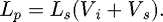 (2)
(2)
An optimised cleaning schedule was also developed in Saudi Arabia [31]. In this study, it was noted that the optimum point varies with cleaning cost and seasonal variation in soiling. Further, an expression was developed that estimates the optimum cleaning frequency.
Despite several studies being attempted to optimise the cleaning frequency in different applications such as domestic, industrial and commercial [1,32], this study seeks to develop an optimisation economic model which determines the cleaning frequency that minimises the unit cost of energy. The study takes into consideration the effect of installation azimuth angle on soiling in the optimisation problem which has not been attempted in previous studies. Further, this work uses an evolutionary optimisation algorithm, a technique that has not been applied before in optimising the cleaning frequency of solar PV collectors. Statistical methods and analytical methods are the techniques that have been used so far in the few studies conducted in this area [17,25,27,31,33,34]. Literature has also shown that an attempt to optimise cleaning frequency using Artificial Neural Networks was made [33]. However, the scarcity of research work in this area has been noted through literature review thus prompting further studies. Evolutionary algorithms have been proven to be able to solve complex optimisation problems in other fields and their application in optimising the cleaning frequency of solar PV collectors is likely to produce even better results than previously generated using other methods.
3 Materials and methods
3.1 Location and data measurement
The study was carried out at a location in Harare, Zimbabwe with co-ordinates 17.8°S and 31.05°E with an altitude of 1490 m. Harare is characterised by mainly low rise buildings with the exception of the central business district (CBD) with high rise buildings with an average of 3–4 floors. The population of Harare was estimated at 2,123,132 from the 2012 census. The measured air particulate matter PM10 and PM2.5 of the city are within the acceptable air quality standards with a mean PM10 of 16.5 μg/m3. The location is classified under tropical savannah climate characterised by two seasons, summer and winter with approximately equal duration in months. Most of the rainfall is experienced in the period from December to February with January the wettest. The dry periods span from May to September with the hottest month being October and the coldest is July which is also the driest (with the least amount of humidity). The month which experiences the most wind is August and the least wind is experienced in January. The 10 year annual average values of the meteorological parameters are shown in Table 1. The location rarely experiences dust storms for the whole year.
PV performance measurements were conducted using 3 × 100W monocrystalline PV collectors (Fig. 1) from January 2018 to December 2018 on a ground mounted facility in an open space with lawn grass located at Harare Institute of Technology (HIT) in Zimbabwe. The PV module characteristics are shown in Table 2. The panels were mounted on the ground for ease of cleaning and dismantling to take the electrical measurements in the lab. The panels were manually cleaned once every month using deionised water and detergents. The cleaning process involved the use of two microfiber wipers for each PV module, one for applying the detergent and removing dirt and the other for rinsing with plenty of water until no visible dirt or spots are seen on the PV collectors.
The PV experimental configurations had a common tilt of 23° and varying azimuth angles of 157.5, 180° and 202.5° representing the directions North of North West (NNW), North (N) and North of North East (NNE) respectively as shown in Figure 1. At the beginning of the experiment, the PV modules were cleaned using de-ionised water to set the transmittance at the highest possible value. Meteorological data including rainfall (mm), wind speed (m/s), relative humidity (%) and wind direction (°) were also measured using a Davis Vantage Pro 2 wireless weather station installed at HIT.
The power, energy and efficiency were calculated using equations (3)–(5) where η, ηr
and β are the efficiency of the solar PV collector, the reference efficiency and the temperature coefficient of the PV collector respectively [35]. Ta
, Tr
and T
NOCT are respectively the ambient temperature, the reference temperature and the nominal cell operating temperature. IT
, Gr
, and P
STC are the hourly solar radiation on a tilted surface, the reference solar radiation and the power output at standard test conditions respectively. (3)
(3)
 (4)
(4)
 (5)
(5)
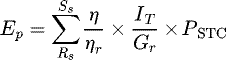
The daily peak power (Pmax), generated by each collector was measured in the evening at 19:00 hrs using a solar simulator with an irradiance of 1000 W/m2 and a temperature of 25 °C. The measured Pmax was used to compute the energy (Ep) generated for the day by making use of the hourly solar irradiance values from sun rise Rs to sunset Ss as shown in equation (4). Other meteorological parameters such as ambient temperature obtained from the weather station at Harare Institute of Technology (HIT) were also used in the computations of the PV operating efficiency as shown in equation (5). (6)
(6)
Other variables measured include the short circuit current (I sc) and open circuit voltage (V oc). The energy was normalised by dividing the recorded value of daily energy by the insolation received on that particular day as shown by equation (6) where En , Ed and Qd are the normalised energy for the ith collector, daily energy generated by the ith PV collector and the insolation received in the particular day respectively. The measured data was also used to determine the soiling ratios which was used in PVSyst simulations to determine the annual energy yield and performance of the PV collectors.
Annual average meteorological values.
 |
Fig. 1 The installation configurations (a) and the weather station (b) used in the study. |
Solar panel characteristics.
3.2 Insolation and annual energy yield
Angstrom's model given in equation (7) [36] was used to compute the annual insolation received by a tilted module at different azimuth angles.  and
and  are respectively the monthly averaged values of the daily global horizontal irradiance and daily extra-terrestrial solar radiation. The constants, k1
and k2
were obtained from previous studies in the same location and their values are 1.0294 and 1.144 respectively [37].
are respectively the monthly averaged values of the daily global horizontal irradiance and daily extra-terrestrial solar radiation. The constants, k1
and k2
were obtained from previous studies in the same location and their values are 1.0294 and 1.144 respectively [37].  , and
, and  are respectively the average monthly values of the daily sunshine hours and the maximum possible daily sunshine hours.
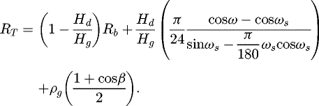
The computation of the radiation on the tilted surface (HT
) and the total tilt factors (RT
) for each PV collector were determined using equations (8) and (9) [36] respectively where the tilt factors for beam, diffuse and reflected irradiance are represented by R
b
, R
d
and R
r
; ρg
is ground reflectivity and for this study it was taken as 0.205.  ,
,  and
and  are respectively the monthly average values of global, beam and diffuse irradiation. H
d
is the diffuse radiation while H
b
is the beam radiation. ω and ω
s
are respectively the hour angle and the sunrise/sunset hour angle for the tilted photovoltaic surface while β is the tilt angle which was taken as 23°.
are respectively the monthly average values of global, beam and diffuse irradiation. H
d
is the diffuse radiation while H
b
is the beam radiation. ω and ω
s
are respectively the hour angle and the sunrise/sunset hour angle for the tilted photovoltaic surface while β is the tilt angle which was taken as 23°. (7)
(7)
 (8)
(8)
 (9)
(9)
3.3 Modelling and optimisation
The soiling ratio (Rs
) was computed for all the modules for each month to evaluate the extent to which soiling had affected the collectors. Equation (10) outlined the computation of (Rs
) where Dr
,
f
and Dr
,l are respectively the relative difference in energy generated for the first day and last day while f and l are the first and last day of the moth respectively.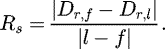 (10)
(10)
An optimisation formulation established by Jones et al. [31] was modified to enable the optimisation using PSO. The model was modified to incorporate the effect of seasonal variations in soiling and differences in azimuth angles. Loss coefficients were also computed for the summer and winter seasons and for each configuration.
The optimum cleaning interval is determined by minimizing the cost per unit energy produced (Ce
) on a single cleaning interval. This cost is a function of maintenance costs (Cm
) and energy production loss (Lp
) where Cm
is made up of the cost of machinery, labour, water and detergents (see Eq. (11)) and in this study the cost of manual cleaning for a 30 kW solar PV plant was taken as $200. Minimising Ce gives the optimum time (t) interval in days for which cleaning should be done. (11)
(11)
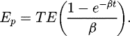
The energy production loss (Lp ) and the value of energy sold (Ep ) are given by equations (12) and (13) [31] where the function L s (t) = 1 − e −βt represents power loss caused by soiling, T is the commercial energy tariff equal to $0.14 for Zimbabwe, E is the energy in kWh produced by a hypothetical 30 kW power plant situated in Harare over a year with 8760 hours in the absence of soiling and β is the energy loss coefficient.
Simulations were also carried out using PVSyst v6.7 to determine the energy generated by a hypothetical 30 kW power plant in a year for each installation configuration taking cognisance of the variations in energy yield and soiling for each configuration. In the simulations, a fixed tilt angle of 23° was used while the azimuth angles were varied between 157.5°, 180° and 202.5° respectively for North of North West (NNW), North (N) and North of North East (NNE) directions. The percentage annual soiling losses were incorporated in the simulation model while the simulation assumed 1.5% losses at Standard Test Conditions (STC). Electrical characteristics data of the 100 Watt PV modules manufactured by Conick were added to the PVSyst list of solar panels data for use in the simulation process.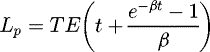 (12)
(12)
 (13)
(13)
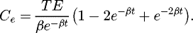
The point at which the energy costs (Ce
) are optimal occurs when the ratio of cost (of energy lost due to soiling and cost of cleaning) to value of energy produced is equal to the ratio of energy loss to energy gain as indicated by equation (14) which is further expanded to equation (15) where the unit cost of energy, Ce
is made the subject.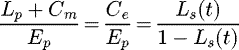 (14)
(14)
 (15)
(15)
Matlab R2018a [38] was used in this optimisation problem with PSO algorithm being employed in the optimisation problem to minimise the unit energy cost Ce . This algorithm has capabilities for both local and global optimisation thus it is capable of retaining the global solution in the search space [39,40]. Owing to its ability to retain the global solution, it has been successfully implemented in minimising the cost per unit power for a wind farm [41] and hence the global version of PSO was used in this study. The PSO algorithm is a metaheuristic optimisation technique which mimics the movement of a flock of birds or a school of fish that are searching for a singular food item. A bird is thus represented as a particle which is a single solution to the optimisation problem. There are two main parameters in PSO which are velocity and position and a particle maintains its individual best position (P best) and the swarm maintains a global best position (G best). The velocity and position are updated using equations (16) and (17) respectively where ω, c 1 and c 2 are constants and rand1() and rand2() are random variables. ω is inertia weight and was taken as 1 while c 1 and c 2 are personal learning coefficient and global learning coefficient and were respectively taken as 1.5 and 2.0. The damping factor ωdamp used in this study was taken as 0.99. The PSO algorithm was run with 75 iterations and a population of 50.
 (16)
(16)
 (17)
(17)
4 Results and discussions
The experimental study revealed that maximum energy was generated at the beginning of the experiment and gradually decreased with time of exposure and the soiling was visually noted to be homogeneous on the solar collector. The amount of soiling was however found to be dependent on the meteorological parameters particularly wind speed, wind direction, ambient temperature and relative humidity as revealed by the varying amount of soiling on a daily basis for each PV collector.
There was a significant improvement in PV performance in the summer season during the experimentation time period from the 1st of January 2018 to 31st March 2018 and from the 25th of October 2018 to 31st December 2018. Meanwhile heavy soiling was experienced during the dry season spanning from May to October with the worst soiling conditions witnessed during the period between July and October.
The amount of precipitation experienced during the period under study was measured and analysed. Light showers of less than 6 mm experienced in the winter especially in June and July did not bring any improvement but rather worsened the situation due to the cementation effect of light rainfall which is similar to that of high humidity and dew [5,16].
4.1 Solar radiation and energy generated
The collectors were facing the general north direction i.e. North of North West (NNW), North (N) and North of North East (NNE) to harvest as much energy as possible since the location is in the southern hemisphere. Transposition factors (Tf
) (see Eq. (18)) which represent the ratio of the incident irradiation on a tilted plane to that on the horizontal surface were determined for the three configurations where Gt
and Gh
are respectively the irradiance on the tilted surface and the irradiance on a horizontal plane. The transposition factor gives an indication of what is lost or gained when the collector plane is tilted. Values greater than one indicate a gain and those less than one indicate a loss in energy generated. Table 3, gives the transposition factors as 1.06, 1.07, and 1.06 respectively, for the three different orientations i.e. NNW, N and NNE and the maximum possible annual insolation received by these collectors were computed respectively as 2015 kWh/m2, 2026 kWh/m2, and 2012 kWh/m2 from the simulation carried out using PVSyst v6.7. The simulation also revealed that the maximum possible annual energy generation without soiling was between 49.0 MWh and 49.6 MWh for the three configurations used. (18)
(18)
The study revealed that for azimuth angles ranging between 157.5° and 202.5°, with other variables being uniform, the maximum possible difference in energy generated is only 1.2% which is practically insignificant. This indicates that an azimuth deviation of up to 12.5% measured from the optimum azimuth angle will yield up to a 1.2% maximum possible energy loss. Such an outcome reveals that if a collector is slightly deviating from the North in the Southern hemisphere, the energy loss is very less and a similar outcome is also expected in the Northern hemisphere.
Transposition factors and maximum possible annual energy yield.
4.2 Soiling losses
Although collectors facing to the north at 180° azimuth theoretically collects the maximum energy in the southern hemisphere, slight deviations may still produce desirable or better results if the effect of soiling is carefully considered and studied. In this study loss coefficients (β) per hour were calculated for each month for the monocrystalline collectors used as shown in Table 4 to evaluate the differences in soiling for different configurations. Annual loss coefficients (×10‑3.25) of 3.14, 2.48 and 1.78 were computed for the configurations North of North East (NNE), North (N) and North of North West (NNW) respectively. The NNW configuration had the least loss coefficient while the NNE had the highest loss coefficient. Making use of the soiling loss Equation L s (t) = 1 − e −βt for the three configurations to represent power loss due to soiling yielded equations (19)–(21) in Table 5.
The computed soiling ratio for each configuration are highlighted in Figure 2. It was found that the average monthly soiling ratios were 10.45%, 8.27% and 5.93% respectively for the configurations North of North East (NNE), North (N) and North of North West (NNW). The results revealed that there was more soiling in the winter with the highest amount of soiling occurring in the month of August. This scenario is attributed to violent winds and high wind speeds associated with this month. Due to the absence of rainfall during winter times, there are high levels of soiling compared to summer season which experiences rainfall at least once every four days on average. This rainfall has a significant cleaning effect thereby reducing the amount of soiling experienced during this season.
The average loss coefficients and soiling ratios for winter and summer seasons are shown in Table 6. From the table, it is evident that the loss coefficients in winter are higher than the loss coefficients in summer and the same applies to the soiling ratios.
Loss coefficients for the three configurations (×10‑3.25).
The derived power loss equations for the three configurations.
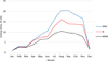 |
Fig. 2 Monthly soiling ratios (%) for the three configurations. |
The average annual, winter and summer loss coefficients and soiling ratios for the three configurations.
4.3 Electrical performance
The computed soiling ratios from the experiments were used to simulate the annual energy production in PVSyst for each configuration. The results indicated that the panels had different annual energy production and performance as given in Table 7. A control panel was added in the simulation process where the soiling was 0% meaning the panel is cleaned every day.
Table 7 shows the differences in annual energy production per each configuration. The NNW configuration had the highest performance with an annual production of 46.4 MWh/year while the NNE configuration had the least energy production of 45.0 MWh/year. The NNE configuration produced 2.2% less energy compared to the collector with an N configuration while the NNW configuration produced 0.87% more energy. However, when the energy production is compared to a control panel that is cleaned on a daily basis, it was noted that the configurations NNE, N and NNW had an annual energy yield difference of 9.27%, 7.25% and 6.45% respectively. The NNW configuration shows the highest performance with a small difference in the annual energy yield. The reason for more energy being generated by this configuration can be attributed to the wind flow characteristics in this location in relation to the orientation of the PV collector. The general wind flow direction in the location as obtained from the measured data is North-East to South-East as shown by the wind rose in Figure 3.
Such a phenomenon will make the collector facing NNE have more direct interactions with the wind while the NNW configuration has less direct interactions with the wind thereby yielding less soiling. This phenomenon was observed in other PV soiling studies [8,42,43].
Electrical performance of the PV collectors at different azimuth angles.
 |
Fig. 3 Wind Rose showing the annual direction of the wind. |
4.4 Optimization of cleaning cycle
From the results highlighted in Table 6, it is evident that the loss coefficients for the winter season are significantly different from the loss coefficients for the summer season. It was therefore concluded that the cleaning cycle optimization was necessary for the winter season only and during summer natural cleaning by rain will be utilised. The energy loss due to soiling for the three configurations for the winter seasons were established as shown by equations (22)–(24) respectively for North of North East (NNE), North (N) and North of North West (NNW) configurations. Bearing this in mind, the optimum cleaning cycle was determined for each configuration by minimizing equation (15) subject to 0 ≤ t ≤183 days for each configuration where the loss coefficients for each configuration are shown by equations (22)–(24) as previously highlighted.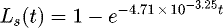 (22)
(22)
 (23)
(23)
 (24)
(24)
The problem was formulated and optimized as shown in Table 8 using PSO algorithm where 0 ≤ t ≤ 183 and t is time in days between cleaning intervals during the dry season where soiling is most common. For example, when t = 0 no cleaning is required at all, when t =1 cleaning is required every day and when t = 183 cleaning is required once in each dry season.
The optimization using the PSO algorithm gave optimized cleaning cycle results for each configuration. The solution converged after an average of 28 iterations for each configuration and Figure 4 shows the 28 iterations for the NNW configuration. The fast convergence (see Fig. 5) shows the good efficiency and superiority of PSO algorithm in optimization problems compared traditional optimization techniques. PSO is able to solve highly complex, non-linear and multidimensional problems and similar conclusions were also outlined in other studies [44,45]. The optimisation results indicated that for the NNE, N and NNW configurations, it is necessary to clean every 18 days, 28 days and 35 days respectively as shown in Table 9.
These results revealed that the NNW configuration gives the least number of cleaning cycles during the dry season and hence it is the most desirable with Ce of $0.093 compared to NNE and N which have a Ce of $0.113 and $0.129 respectively. It is interesting to note that the minimum Ce occurs at different cleaning frequencies for different configurations as outlined in Figure 4 and Table 9. The NNW configuration has the least cost of energy as well as the longest interval between cleaning while the NNE configuration has the highest cost of energy and the shortest cleaning interval.
The result has shown that installation configuration plays a big role in reducing the maintenance costs in terms of cleaning and hence reduces the unit energy cost. The unit cost of energy was found to be reduced by 17.7% by adopting the NNW configuration which offers less soiling thereby reducing maintenance costs. This notable reduction of the cost of energy from the commercial tariff of $0.14 shows the superiority of the PSO algorithm in optimisation of energy problems when compared to similar studies [28,31] which used traditional approaches in solving the optimisation problem.
A comparison of PSO with the analytical method was done and it was found that there was a good correlation of the results between the two methods as shown in Figure 6. A high coefficient of determination (R 2) was found and it was 98.9%. The mean absolute percentage error (MAPE) and the residual mean square errors were found to be 1.96% and $0.0197 respectively. The analytical method was however found to give results which are slightly higher than the PSO algorithm. This is because the analytical method when used for this particular problem has fixed predetermined steps which are more of trial and error to get the minimum value.
Using this method, the minimum unit cost of energy was found to be $0.12 with a cleaning frequency of 29 days. The cost was about 29% higher than the minimum cost determined from the PSO algorithm. This difference indicate that even a slight difference of the minimized value of the unit cost of energy has a huge effect on the overall cost of energy when expressed as a percentage. For a big power plant, a difference of 29% in revenues signifies a huge loss thus the PSO method proved to be an indispensable tool that can minimize cost to desirable levels when compared to manual optimization techniques.
Although Figure 6 gives a good correlation, it should be noted that the PSO algorithm has a good performance in terms of minimization of the unit cost of energy compared to the analytical method. The PSO algorithm converges after 28 iterations while the manual method required the substitution of all days from day 1 to day 365 into the objective function in steps of one to compute all the possibilities in a full year of 365 days which is laborious. This signifies a 92% faster convergence of PSO compared to the manual method and hence it warrants its use in huge and complicated energy optimization problems.
Optimisation problem formulation for the three configurations.
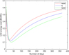 |
Fig. 4 Minimised unit energy cost and the cleaning frequency. |
 |
Fig. 5 Solution convergence diagram for NNW configuration. |
Optimisation results.
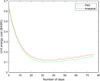 |
Fig. 6 Comparison of PSO with the analytical method. |
5 Conclusions
The importance of installation configuration in optimising the cleaning cycle and hence reduce the unit cost of energy was explored in this research. It was noted that if a proper orientation is selected as opposed to the general North for the southern hemisphere, the cost of energy can be significantly reduced due to reduced soiling rate and thus reducing the maintenance costs. The study revealed that the azimuth of 180° for the southern hemisphere is not always the best azimuth if soiling issues are taken into consideration. It is therefore required to take cognisance of the soiling effects in determining the best installation azimuth for any location. The NNW configuration was found to be the best location with a soiling ratio of 5.93% compared to 8.27% for the N configuration. Although the N configuration receives more solar radiation, the effect is counter acted by more soiling experienced. The study revealed a maximum theoretical difference in annual energy yield of 1.2% while the difference in soiling was found to be 28.29% indicating the need to recognise the significant effect of soiling in determining the optimum installation azimuth angle.
References
- J. Tanesab, D. Parlevliet, J. Whale, T. Urmee, Energy and economic losses caused by dust on residential photovoltaic (PV) systems deployed in different climate areas, Renew. Energy 120 , 401–412 (2018) [CrossRef] [Google Scholar]
- G. Picotti, P. Borghesani, G. Manzolini, M.E. Cholette, R. Wang, Development and experimental validation of a physical model for the soiling of mirrors for CSP industry applications, Sol. Energy 173 , 1287–1305 (2018) [CrossRef] [Google Scholar]
- K. Ilse, M. Werner, V. Naumann, B.W. Figgis, C. Hagendorf, J. Bagdahn, Microstructural analysis of the cementation process during soiling on glass surfaces in arid and semi-arid climates, Phys. Status Solidi 10 , 525–529 (2016) [Google Scholar]
- M. García, L. Marroyo, E. Lorenzo, M. Pérez, Soiling and other optical losses in solar-tracking PV plants in navarra, Prog. Photovolt. Res. Appl. 19 , 211–217 (2011) [CrossRef] [Google Scholar]
- T. Sarver, A. Al-Qaraghuli, L.L. Kazmerski, A comprehensive review of the impact of dust on the use of solar energy: history, investigations, results, literature, and mitigation approaches, Renew. Sustain. Energy Rev. 22 , 698–733 (2013) [CrossRef] [Google Scholar]
- H. Hottel, B. Woertz, Performance of flat-plate solar-heat collectors, Trans. ASME Am. Soc. Mech. Eng. U.S.A. 64 (1942) [Google Scholar]
- H.P. Garg, Effect of dirt on transparent covers in flat-plate solar energy collectors, Sol. Energy 15 , 299–302 (1974) [CrossRef] [Google Scholar]
- I.I. Mailuha, H. Murase, Knowledge engineering-based studies on solar energy utilization in Kenya, Agric. Mech. Asia Afr. Lat. Am. 25 , 13–6 (1994) [Google Scholar]
- S.A.M. Said, Effects of dust accumulation on performances of thermal and photovoltaic flat-plate collectors, Appl. Energy 37 , 73–84 (1990) [CrossRef] [Google Scholar]
- B. Nimmo, S.A.M. Said, Effects of dust on the performance of thermal and photovoltaic flat plate collectors in Saudi Arabia − preliminary results 1 , 145–152 (1981) [Google Scholar]
- A.M. El-Nashar, The effect of dust accumulation on the performance of evacuated tube collectors, Sol. Energy 53 , 105–115 (1994) [CrossRef] [Google Scholar]
- A.A. Hegazy, Effect of dust accumulation on solar transmittance through glass covers of plate-type collectors, Renew. Energy 22 , 525–540 (2001) [CrossRef] [Google Scholar]
- J.K. Kaldellis, A. Kokala, Quantifying the decrease of the photovoltaic panels' energy yield due to phenomena of natural air pollution disposal, Energy 35 , 4862–4869 (2010) [CrossRef] [Google Scholar]
- D. Goossens, Z.Y. Offer, A. Zangvil, Wind tunnel experiments and field investigations of eolian dust deposition on photovoltaic solar collectors, Sol. Energy 50 , 75–84 (1993) [CrossRef] [Google Scholar]
- D. Goossens, E. van Kerschaever, Aeolin dust deposition on photovoltaic solar cells: the effects of wind velocity and airborne dust concentration on cell performance, Sol. Energy 66 , 277–289 (1999) [CrossRef] [Google Scholar]
- H.K. Elminir, A.E. Ghitas, R.H. Hamid, F. El-Hussainy, M.M. Beheary, K.M. Abdel-Moneim, Effect of dust on the transparent cover of solar collectors, Energy Convers. Manag. 47 , 3192–3203 (2006) [Google Scholar]
- E.G. Luque, F. Antonanzas-Torres, R. Escobar, Effect of soiling in bifacial PV modules and cleaning schedule optimization, Energy Convers. Manag. 174 , 615–625 (2018) [CrossRef] [Google Scholar]
- A. Syafiq, A.K. Pandey, N.N. Adzman, N. A. Rahim, Advances in approaches and methods for self-cleaning of solar photovoltaic panels, Sol. Energy 162 , 597–619 (2018) [CrossRef] [Google Scholar]
- Z. Chen, R. Xiong, J. Cao, Particle swarm optimization-based optimal power management of plug-in hybrid electric vehicles considering uncertain driving conditions, Energy 96 , 197–208 (2016) [CrossRef] [Google Scholar]
- H. Ajdad, Y. Filali Baba, A. Al Mers, O. Merroun, A. Bouatem, N. Boutammachte, Particle swarm optimization algorithm for optical-geometric optimization of linear fresnel solar concentrators, Renew. Energy 130 , 992–1001 (2019) [CrossRef] [Google Scholar]
- M.G. Carneiro, R. Cheng, L. Zhao, Y. Jin, Particle swarm optimization for network-based data classification, Neural Netw. 110 , 243–255 (2019) [CrossRef] [Google Scholar]
- Z. Liu, C. Zhu, P. Zhu, W. Chen, Reliability-based design optimization of composite battery box based on modified particle swarm optimization algorithm, Compos. Struct. 204 , 239–255 (2018) [CrossRef] [Google Scholar]
- G. Xu, G. Yu, On convergence analysis of particle swarm optimization algorithm, J. Comput. Appl. Math. 333 , 65–73 (2018) [CrossRef] [Google Scholar]
- H. Zhou, J. Pang, P.-K. Chen, F.-D. Chou, A modified particle swarm optimization algorithm for a batch-processing machine scheduling problem with arbitrary release times and non-identical job sizes, Comput. Ind. Eng. 123 , 67–81 (2018) [CrossRef] [Google Scholar]
- P. Besson, C. Muñoz, G. Ramírez-Sagner, M. Salgado, R. Escobar, W. Platzer, Long-term soiling analysis for three photovoltaic technologies in Santiago region, IEEE J. Photovolt. 7 , 1755–1760 (2017) [CrossRef] [Google Scholar]
- E. Urrejola et al., Effect of soiling and sunlight exposure on the performance ratio of photovoltaic technologies in Santiago, Chile, Energy Convers. Manag. 114 , 338–347 (2016) [CrossRef] [Google Scholar]
- Y. Jiang, L. Lu, H. Lu, A novel model to estimate the cleaning frequency for dirty solar photovoltaic (PV) modules in desert environment, Sol. Energy 140 , 236–240 (2016) [CrossRef] [Google Scholar]
- E. Fuentealba, P. Ferrada, F. Araya, A. Marzo, C. Parrado, C. Portillo, Photovoltaic performance and LCoE comparison at the coastal zone of the Atacama Desert, Chile, Energy Convers. Manag. 95 , 181–186 (2015) [CrossRef] [Google Scholar]
- L. Cristaldi et al., Economical evaluation of PV system losses due to the dust and pollution, in 2012 IEEE International Instrumentation and Measurement Technology Conference Proceedings , May 2012, pp. 614–618, doi: 10.1109/I2MTC.2012.6229521 [CrossRef] [Google Scholar]
- M. Faifer, M. Lazzaroni, S. Toscani, Dust effects on the PV plant efficiency: a new monitoring strategy 580–585 (2014) [Google Scholar]
- R.K. Jones et al., Optimized cleaning cost and schedule based on observed soiling conditions for photovoltaic plants in Central Saudi Arabia, IEEE J. Photovolt. 6 , 730–738 (2016) [CrossRef] [Google Scholar]
- J. Tanesab, D. Parlevliet, J. Whale, T. Urmee, Dust effect and its economic analysis on PV modules deployed in a temperate climate zone, Energy Proc. 100 , 65–68 (2016) [CrossRef] [Google Scholar]
- B. Hammad, M. Al-Abed, A. Al-Ghandoor, A. Al-Sardeah, A. Al-Bashir, Modeling and analysis of dust and temperature effects on photovoltaic systems' performance and optimal cleaning frequency: Jordan case study, Renew. Sustain. Energy Rev. 82 , 2218–2234 (2018) [CrossRef] [Google Scholar]
- H. Truong Ba, M.E. Cholette, R. Wang, P. Borghesani, L. Ma, T.A. Steinberg, Optimal condition-based cleaning of solar power collectors, Sol. Energy 157 , 762–777 (2017) [CrossRef] [Google Scholar]
- S. Dubey, J.N. Sarvaiya, B. Seshadri, Temperature dependent photovoltaic (PV) efficiency and its effect on PV production in the world − a review, Energy Proc. 33 , 311–321 (2013) [CrossRef] [Google Scholar]
- S.P. Sukhatme, J.K. Nayak, Solar energy: principles of thermal collection and storage , 3rd ed. (Tata McGraw-Hill, New Delhi, 2008) [Google Scholar]
- T. Hove, J. Göttsche, Mapping global, diffuse and beam solar radiation over Zimbabwe, Renew. Energy 18 , 535–556 (1999) [CrossRef] [Google Scholar]
- MathWorks − Makers of MATLAB and Simulink. https://www.mathworks.com/ (accessedMay 15, 2020) [Google Scholar]
- R.-J. Ma, N.-Y. Yu, J.-Y. Hu, Application of particle swarm optimization algorithm in the heating system planning problem, Sci. World J. 2013 , 1–11 (2013) [Google Scholar]
- D. Wang, D. Tan, L. Liu, Particle swarm optimization algorithm: an overview, Soft Comput. 22 , 387–408 (2018) [CrossRef] [Google Scholar]
- V. Aristidis, P. Maria, L. Christos, Particle swarm optimization (PSO) algorithm for wind farm optimal design, Int. J. Manag. Sci. Eng. Manag. 5 , 53–58 (2010) [Google Scholar]
- D. Goossens, Z.Y. Offer, A. Zangvil, Wind tunnel experiments and field investigations of eolian dust deposition on photovoltaic solar collectors, Sol. Energy 50 , 75–84 (1993) [CrossRef] [Google Scholar]
- M. Mani, R. Pillai, Impact of dust on solar photovoltaic (PV) performance: research status, challenges and recommendations, Renew. Sustain. Energy Rev. 14 , 3124–3131 (2010) [Google Scholar]
- I. Boussaïd, J. Lepagnot, P. Siarry, A survey on optimization metaheuristics, Inf. Sci. 237 , 82–117 (2013) [CrossRef] [MathSciNet] [Google Scholar]
- M. Madi, Comparison of meta-heuristic algorithms for solving machining optimization problems, Facta Univ. Ser. Mech. Eng. 11 , 29–44 (2013) [Google Scholar]
Cite this article as: K. Chiteka, R. Arora, S.N. Sridhara, C.C. Enweremadu, Cleaning cycle optimisation in non-tracking ground mounted solar PV systems using Particle Swarm Optimisation, Int. J. Simul. Multidisci. Des. Optim. 11, 9 (2020)
All Tables
The average annual, winter and summer loss coefficients and soiling ratios for the three configurations.
All Figures
|
Fig. 1 The installation configurations (a) and the weather station (b) used in the study. |
| In the text | |
|
Fig. 2 Monthly soiling ratios (%) for the three configurations. |
| In the text | |
|
Fig. 3 Wind Rose showing the annual direction of the wind. |
| In the text | |
|
Fig. 4 Minimised unit energy cost and the cleaning frequency. |
| In the text | |
|
Fig. 5 Solution convergence diagram for NNW configuration. |
| In the text | |
|
Fig. 6 Comparison of PSO with the analytical method. |
| In the text | |
Current usage metrics show cumulative count of Article Views (full-text article views including HTML views, PDF and ePub downloads, according to the available data) and Abstracts Views on Vision4Press platform.
Data correspond to usage on the plateform after 2015. The current usage metrics is available 48-96 hours after online publication and is updated daily on week days.
Initial download of the metrics may take a while.