


| Issue |
Int. J. Simul. Multidisci. Des. Optim.
Volume 17, 2026
|
|
|---|---|---|
| Article Number | 12 | |
| Number of page(s) | 9 | |
| DOI | https://doi.org/10.1051/smdo/2025035 | |
| Published online | 11 June 2026 | |
Research Article
Determining the equilibrium distribution state of fluidic molecule model
School of Mechanical and Automotive Engineering, Ha Noi University of Industry, No 298, Cau Dien Street, Bac Tu Liem District, Hanoi City, Vietnam
* e-mail: This email address is being protected from spambots. You need JavaScript enabled to view it.
Received:
2
December
2024
Accepted:
7
November
2025
Abstract
This study employs the C++ programming framework and Tecplot software to construct the initial fluidic molecular structure model. A molecular dynamics simulation method is utilized to modify the molecular structure during a prerun process, aiming to establish the natural equilibrium state of molecules that aligns with the Maxwell-Boltzmann distribution plot. The 3D model representing the natural equilibrium fluidic state, developed after the pre-run process, is used to explore fluidic nanojet ejections under various technological parameters. The outcomes of the fluidic nanojets obtained through the simulation process reveal disparities under different research scenarios such as pressing forces, system temperatures, and nozzle diameters. These acquired fluidic nanojets further validate the credibility of the established natural equilibrium state after the 10,000 femtosecond (fs) pre-run process, thus serving as a reliable foundation for subsequent investigations based on this fundamental equilibrium premise. Furthermore, this study provides significant insights into the dynamic ejection of fluidic nanojets through molecular dynamics simulations. Additionally, the generated data are invaluable for experimental endeavors and manufacturing processes incorporating this technology.
Key words: Molecular dynamics simulation / fluidic molecule structure model / natural molecule statement / fluidic nanojet ejection
© V.Q. Nguyen et al., Published by EDP Sciences, 2026
 This is an Open Access article distributed under the terms of the Creative Commons Attribution License (https://creativecommons.org/licenses/by/4.0), which permits unrestricted use, distribution, and reproduction in any medium, provided the original work is properly cited.
1 Introduction
The growing demand for optimizing nano-sized equipment has led to widespread applications in various industrial sectors, such as mechanical machining, lubrication, printed circuit board manufacturing, and liquid nanojet ejection technology. In addition, this technology is used for dispensing biological reagents, 3D prototyping, and microelectrical wiring [1,2].
Research content has focused on fluid nanojet formation and nanoscale droplet separation, crucial for designing and operating nanoscale devices. Otherwise, advances in the mechanical machining lubrication area are discussed, and performance-oriented [3,4].
Using dynamic simulations, researchers have investigated the ejection of water molecules through reservoir nozzles under external forces. The effects of pressing forces have also been analyzed, showing that the dynamics of nanoscale liquid jets can be accurately captured. The breakup dynamics of droplets from fluid jets have been explored, influenced by factors like temperature and aperture shapes [5,6].
Molecular dynamics (MD) simulations have been widely used to examine for various technology parameters, including nozzle diameters, pressing forces and fluid properties. The simulation results show clearly insights into nano water droplet performing and argon cluster evaporation phenomena [7–11].
MD analyses also reveals that temperature affects the spreading of droplets deposition on solid plates. Water nanojet formation through nano-orifices and impingement on flat surfaces is scrutinized [12].
Empirical methods are employed to study nanoscale fluid droplet impingement, coalescence, and collisions on flat surfaces. However, the natural equilibrium state of molecules has received limited attention [13].
This research builds on previous MD simulations of water nanojet ejection to estimate the natural equilibrium distribution of fluid molecules after a pre-run process [14–19]. This foundational step enhances subsequent simulation research under varying technological parameters, aim for desired outcomes.
2 Research approach
2.1 The simulation tool
Molecular dynamics (MD) is a powerful tool for molecular modeling, facilitating the study of molecular motion. Through simulating molecular interactions, we aim to comprehend assembly properties in relation to structure and dynamic system evolution over a defined time frame. Typically, Newton’s equations dictate the molecule trajectories for interacting particles in a system.
Given the complexity of molecular systems composed of numerous particles, MD simulations are pivotal in uncovering their properties [20]. We delve into the two most prevalent methods, energy minimization and molecular dynamics. These methods simulate the optimal structure and inherent motion of molecules to determine suitable simulation parameters and energy minimization. Additionally, the section elaborates on techniques for analyzing simulations, including potential energies, geometric attributes, structural fluctuations, and coordinate stability.
2.2 The molecular interactions
Molecular dynamics simulation orchestrates molecular interactions using numerical methods, step-by-step progression, and resolution of classical motion equations. This methodology is applicable even to basic molecular systems, as shown in equation (1):
 (1)
(1)
The force components fi which act on the molecules needs to be considered to derive the potential energies of u(rN), with rN=(r1, r2, … rN) is a molecule coordinate set. The potential energy function u(rN) focuses for describing the molecular interactions.
2.3 The molecule interactions
The potential energy unon−bonded is used to represent the function of non-bonded interactions between molecules, as shown in equation (2):
 (2)
(2)
Where the term of the externally applied potential is ur which often has concentrated on the pair potential v(ri, rj)
In simulations of complex fluids, basic models are often employed to capture essential physics. This research specifically emphasizes differential and continuous pair potentials. The Lennard-Jones potential, typically in its common form, is widely utilized, as shown in equation (3):
 (3)
(3)
With the diameter and well depth signs are σ and ℰ, respectively.
The appropriate Coulomb potentials is added to present for the electrostatic charges, as follows in equation (4):
 (4)
(4)
Where the charges and permittivity of free space are Q1, Q2 and ℰ0, respectively.
2.4 Calculating the force in the molecular dynamics interactions
In molecular dynamics impactions, the force computation is extremerly complex and consumes a significant amount of computational time. Enhancing force calculations involves various techniques, which have two main objectives: reducing the number of particles considered in the interaction potential and minimizing the time spent locating particles within the range of molecular interaction of calculating the forces.
Usually, forces originate from interactions among particles. However, particles that are far apart result in weaker forces. The potential compensates for material has form shown in the equation (5).
 (5)
(5)
Where rc is material outside of the cutoff radius and ρ is average density of the system [16].
Periodic boundary conditions are utilized as a substitute for potential truncation which each particle in the system is obtained by shifting particle positions along the periodic boundaries. The distance of particles A and B is represented as in the equation (6):
 (6)
(6)
The particles A and B have the position vectors of rA and rB, respectively, the lattice vectors along periodic boundaries are m and n, respectively.
The potential function is truncated using the cutoff method. This technique is also employed to determine the distance between pairs of particles that cross the boundary. The cutoff method is directly used to compute the force between other particles. However, force calculations are restricted to particles within the cutoff radius. This selection proces can become time-consuming, especially when dealing with a significant number of particles.
The force which has the impaction of the particles are calculated as the requirement with  . Meanwhile, when N is very large, the computational cost is enormous.
2.5 The MD algorithm
Today, the molecular dynamics algorithm is widely utilized, even though Newton’s equations have been known. This research emphasizes the utilization of numerical algorithms for conducting molecular dynamics simulations.
a The Verlet algorithm
In molecular dynamics, the Newtonian equations of motion are used to numerically integrate for the different finites. However, the selection of suitable algorithms is limited when the system involves a large number of particles.
The Verlet algorithm boasts several advantageous traits, including high speed and strong energy conservation. Verlet first applied this algorithm to a Lennard-Jones system [21]. The initial form of the Verlet algorithm is calculated as equation (7):
 (7)
(7)
where the particle has the values:  with fi(t) is the total force and δ t is the time step for each integration.
The additional finite difference formula is used to determine the velocity of each particle along the trajectories as equation (8):
 (8)
(8)
In the reality, a more convenient approach is to implement a variation of the Verlet algorithm known as the velocity Verlet. The velocity Verlet is presented below as equations (9) and (10):
 (9)
(9)
 (10)
(10)
The Verlet algorithm is adopted for equivalent performance to the original form which is verified by changing the velocity as in equation (11):
 (11)
(11)
The entire algorithm of velocity Verlet includes three steps in programming. Formula (12) provides the first calculation for each interaction ri(t+δt). Second, the part of velocity vi(t+δ t) is determined as,
 (12)
(12)
Finally, the other velocity parameter vi(t+δt) with the newly force is calculated though equation (10) to obtain the entire vi(t+δt) as equation (13):
 (13)
(13)
The algorithm of velocity Verlet is the most advantages method for improving the accuracy in calculating the velocity value.
b Constraints
The constrained bonds are maintained at the constant length through the Lagrangian or Hamiltonian formalisms [18,19]. With the fixed bond length between two atoms of b and the constraint equation can be formulated as follows equation (14):
 (14)
(14)
and the calculation the time derivative of constraint is performed as equation (15):
 (15)
(15)
the constraint forces which act on the atoms are expressed in the Lagrangian formular as:

with Λ is the undetermined multiplier as:

The following scheme is desired to solve which combines (p1, p2) into p and (r1, r2) into r. With simplicity calculation is showed as the equations (16), (17) and (18):
 (16)
(16)
 (17)
(17)
With λ is chosen as: 0=χ(r(t+δt))
 (18)
(18)
With λ is chosen as: 0=χ(r(t+δt), r(t+δt))
It’s crucial to understand that rigidly constrained bond lengths within a simulation system do not encompass the entirety of the simulation process. In lieu of constraints, intra-molecular bond potentials are preserved, and the rapid degrees of freedom is handled by the time step.
c Period boundary condition
The period boundary condition (PBCs) is a boundary condition set which is adropted in computer simulation programs and mathematical models to predict and analyze the properties of extensive systems. Molecules tend to gather near the boundary surfaces of the simulation box in these systems. As a result, surface effects influence these molecules during calculations. These effects become negligible as the system size becomes exceptionally large, and a technique is employed to mitigate surface influences in calculations. PBCs are applied to effectively counteract surface effects on molecules regardless of system size.
As Figure 1 shows that a particle moves out the boundary condition which is an image particle will move into for replacing it.
 |
Fig. 1 Period boundary condition. |
2.6 Building the research model
The initial model in this research is established by employing programing C++ and the molecular dynamics method which is used to avaluate the inherent equilibrium state of fluidic molecules. The interactions among atoms inside molecules are determined using the extra-molecular potential. The interactions among mechanic atoms with fluidic molecules are characterizing by adopting the Spohr potential function. LAMMP programing is utilized to to perform the simulation process for molecular amalgamation and model components.
The model of the molecular dynamics structure is illustrated as in Figure 2. The model encompasses 20,691 molecules, resulting in the molecular density of 0.999972 g/cm3. A lattice constant of a =3.104 Å is used for established the oxygen atom structure which arranges in a simple cubic crystal lattice. The bottom and top plates which both have the thickness of 8.152 Å are used to contain the molecule inside. The plates are made of Au atoms which are arranged into the FCC crystal lattice structures with the lattice constant of 4.076 Å. The period boundary condition is applied following the x - and y -directions. The the nozzle and back plate define the space for containing the fluidic molecules with a separation of 60.872 Angstrom (Å). The fluidic dimension in both the x - and y -directions is 101.9 Å.
The gold atom is adropted for constructing the nozzle and back plates and the lattice constant of a = 4.076 Å is used for these paltes in the structure of face-centered cubic crystal lattice. Each plates contructs 5 layers of atoms with the thickness of 8.152 Å.
Upon completing the model with the aforementioned conditions, a preliminary run is conducted with a simulation duration of 10,000 (fs) and a system temperature of 310 Kelvin. This preliminary phase aims to establish the natural equilibrium state of water molecules within the reservoir. Subsequently, this equilibrium molecular model is employed for various studies under different technological conditions, relevant to diverse fields such as printing technology and electronic circuits.
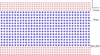 |
Fig. 2 Molecule structure model. |
3 Results and discussion
3.1 The pre-run simulation result
After the pre-run simulation process, the results reveal that initially, water molecules are arranged in a configuration resembling flowers within the structure [18,19]. Nevertheless, this arrangement becomes disrupted after the simulation process, as depicted in Figure 3.
 |
Fig. 3 Molecular dynamics model after pre-run process. |
3.2 The pre-run time follows the Maxwell-Boltmann distribution
To evaluate the adequacy of estimating the natural equilibrium state of water molecules, this outcome is juxtaposed with the Maxwell-Boltzmann criteria distribution function.
Assuming the distribution of molecular particles within the system has achieved equilibrium post the pre-run process, the Maxwell-Boltzmann distribution [20,21] is employed to compute the velocity distribution of molecules subsequent to this initial time step. This distribution depends on the system’s temperature and the mass of the molecular particles. The Maxwell-Boltzmann equation is formulated as follows:
 (19)
(19)
With m is the molecular particle mass, T is the thermodynamic temperature, k is the product of Boltzmann’s constant, V is the velocity of Maxwell function.
Where the velocity components are expressed as equation (20):
 (20)
(20)
The unit of the Maxwell velocity distribution is m/s.
A probability distribution of particle speeds demonstrates the random selection of speeds from the particle population. This distribution is influenced by the system’s temperature and the mass of the particles. As per the Maxwell-Boltzmann equation, the graphical representation of the Maxwell-Boltzmann distribution function displays the shape depicted in Figure 4.
In this study, the initial arrangement of fluidic molecules was structured in the simple cubic crystal lattices which has the lattice constant of 3.104 Å. To ensure natural state of the molecules before initiating the ejection of water molecules from the reservoir, a preliminary run lasting 10,000 fs was conducted for each simulation to achieve an equilibrium state. During this pre-run period, the molecules exhibited chaotic motion within the reservoir.
The velocity distribution of water molecules after the pre-run process is illustrated in Figure 5. The plot of the velocity distribution following the 10,000 fs pre-run period closely resembles the Maxwell-Boltzmann distribution plot depicted in Figure 4. This substantiates that the water molecules display sufficient disorder to attain an equilibrium state during the 10,000 fs pre-run phase.
 |
Fig. 4 Plot of the Maxwell-Boltzmann distribution function. |
 |
Fig. 5 The fluid molecule distribution after the pre-run time of 10000 fs. |
3.3 Water nanojet ejection result
Water nanojet ejection model 3D
The 3D model of the inherent equilibrium state of water is presented in Figure 6. The model comprises three main segments: the nozzle, back plate, and water molecules. The water molecules are confined within the space situated between the nozzle and back plates.
The simulation technology parameters have been established as detailed in Table 1. Three simulation cases will be conducted to expel the water nanojet under uniform conditions, with a nozzle aperture diameter of 40 Å, a system temperature of 310 K, and three different magnitudes of pressing force: 9.0 × 10⁻¹⁰, 10.0 × 10⁻¹⁰ and 11.0 × 10⁻¹⁰ N.
After a simulation time of 150000 fs, the generated water molecule nanojet ejections exhibit variations in terms of length, shape, and diameter across the different simulation scenarios. These differences are influenced by the applied pressing forces.
Snapshots of the water nanojets corresponding to various pressing forces at 150,000 fs are shown in Figure 7. Figures 7a-c show the snapshots of the water nanojets ejected through 40−Å-diameter nozzle aperture with the different pressing forces of 9.25 × 10⁻¹⁰, 10.0 × 10⁻¹⁰, and 11.0 × 10⁻¹⁰ N, respectively under the system temperature of 310 K.
The water nanojets were obtained as shown in Figure 7 shows that the natural equilibrium water statement after pre-run time of 10,000 fs is good enough for using this molecular model performs the other investigations.
 |
Fig. 6 The natural equilibrium water statement model 3D. |
Simulation scheme.
 |
Fig. 7 Snapshots of the water nanojet at 150,000 fs. (a)-(c) Water nanojets of the 40−Å-diameter nozzle aperture for various pressing forces. |
4 Conclusions
This paper employed the molecular dynamics simulation method to explore the state of natural equilibrium of water molecules after a pre-run process. The key conclusions are summarized as follows:
The initial water structure model underwent a pre-run process of 10,000 fs at a system temperature of 310 K to establish the natural equilibrium state of water molecules within the reservoir.
Subsequent to the pre-run simulation process, the results revealed that the water molecules underwent restructuring to achieve a natural equilibrium state that closely aligns with the Maxwell-Boltzmann distribution plot.
The 3D model representing the natural equilibrium water state, developed after the pre-run process, was employed to investigate water nanojet ejections under various technological parameters, including nozzle size, system temperature, and pressing forces.
The water nanojets obtained after a simulation period of 150,000 fs displayed disparities in terms of length, shape, and diameter across the different simulation scenarios.
The acquired water nanojets also validate that the established natural equilibrium state after the pre-run process of 10,000 fs serves as an accurated foundation for further investigations based on this fundamental equilibrium statement.
Acknowledgments
This research was partially supported by the Department of Sciences and Technology, Hanoi University of Industry, Vietnam.
Conflicts of interest
The authors declare no conflict of interest.
Funding
This research is supported by Department of Sciences and Technology, Hanoi University of Industry, Viet Nam.
Data availability statement
The data supporting the findings of this study are available from the corresponding author upon reasonable request.
Author contribution statement
Van Quang Nguyen: Parameter investigation, Using software, Methodology, Data analysis, Visualization Conceptualization, Data curation. Van Thien Nguyen: Funding acquisition, Project administration, Resources, Validation, Writing - review & editing. Ta Thi Tra Giang: Writing - original draft, Visualization Conceptualization, Writing - review & editing.
References
- Q.N. Van, T.N. Van, D.H. Tien, Investigating the influential factors of ejective time and compressible force magnitude to fluid jet movement, Int. J. Simul. Multidisci. Des. Optim. 12, 1–3 (2021). [CrossRef] [EDP Sciences] [Google Scholar]
- T. Ramesh, A.S. Praveen, P.B. Pillai, Numerical simulation of heat sinks with different configurations for high power LED thermal management, Int. J. Simul. Multidisci. Des. Optim. 13, 18 (2022). [Google Scholar]
- Q. Li, C. Liu, Molecular dynamics simulation of heat transfer with effects of fluid-lattice interactions, Int. J. Heat Mass Transfer. 55, 8088–8092 (2012). [Google Scholar]
- Q. Jiasheng, F.A. Gilmar, Z. Xuehua, Surface nanodroplets: formation, dissolution, and applications, Langmuir, 35, 39, 12583–12596 (2019). [CrossRef] [Google Scholar]
- M. Jia, B.Y. Jae, Z. Xuehua, Viscosity-mediated growth and coalescence of surface nanodroplets, J. Phys. Chem. C, 124, 23, 12476–12484 (2020). [CrossRef] [Google Scholar]
- A. Suphanat, Y.M. A. Elisa, Y. Jingjie, Y.N. Teng, Many-body dissipative particle dynamics simulations of nanodroplet formation in 3D nano-inkjet printing, Modell. Simul. Mater. Sci. Eng. 27, (2019). [Google Scholar]
- T.T. Fu, Y.N. Wu, Y.G. Ma, Droplet formation and breakup dynamics in microfluidic flow-focusing devices: From dripping to jetting, Chem. Eng. Sci. 84, 207–217 (2012). [Google Scholar]
- Q.N. Van, S.P. Xuan, W.L. Jau, Separation criteria of nanoscale water droplets from a nozzle plate surface, MATEC Web Conf. 169, 01016 (2018). [Google Scholar]
- N.S.R. Krishnan, S.P. Uppu, A novel approach for noise prediction using Neural network trained with an efficient optimization technique, Int. J. Simul. Multidisci. Des. Optim. 14, 3 (2023). [Google Scholar]
- H.H. Bao, C.L. Bin, B.L. Yao, Molecular dynamics simulations of the nano-droplet impact process on hydrophobic surfaces, Chin. Phys. B. 23, 074702 (2014). [Google Scholar]
- R. Chen et al., Statistical validation methods for nanoscale simulations, Comput. Mater. Sci. 190, 110307 (2021). [Google Scholar]
- Q.N. Van, W.L. Jau, Investigation of temperature effects on nanoscale water droplet separation onto a fixed solid plate, Simul.: Trans. Soc. Model. Simul. Int. 1-9 (2016). [Google Scholar]
- A. Dalili, S. Chandra, J. Mostaghimi, Formation of liquid sheets by deposition of droplets on a surface, J. Colloid Interface Sci. 418, 292–299 (2014). [CrossRef] [Google Scholar]
- T.T.B. Ngo, V.T. Nguyen, T.H. Fang, Nanoscale friction behavior and deformation during copper chemical mechanical polishing process, J. Mol. Model. 29, 293 (2023). [Google Scholar]
- M. Liu et al., Advanced optimization methods in MD-based fluid simulations, J. Nanofluids, 12, 1162–1171 (2023). [Google Scholar]
- A. Zhang et al., Optimized MD simulation of nanoscale jet formation, Nano Lett. 19, 8901–8908 (2019). [Google Scholar]
- V.Q. Nguyen, J.W. Lin, V.D. Pham, Studying the influences of temperature to the liquid ejection and nanodroplet formation, Int. J. Nanosci. 19, 06 (2020). [Google Scholar]
- M. Jia, B.Y. Jae, Z. Xuehua, Viscosity-mediated growth and coalescence of surface nanodroplets, J. Phys. Chem. C, 124, 23, 12476–12484 (2020). [Google Scholar]
- Y. Kim, H. Lee, Equilibrium analysis of molecular dynamics in confined systems, J. Mol. Liquids, 314, 113588 (2020). [Google Scholar]
- S.S. Masatsugu, Maxwell-Boltzmann distribution function (Department of Physics, SUNY at Binghamton, 2012), pp. 1–24. [Google Scholar]
- H. Hugo, Standard Maxwell-Boltzmann distribution: definition and Properties, ForsChem Res. 2, 1–16 (2017). [Google Scholar]
Cite this article as: Van Quang Nguyen, Van Thien Nguyen, and Ta Thi Tra Giang, Determining the equilibrium distribution state of fluidic molecule model, Int. J. Simul. Multidisci. Des. Optim. 17, 12 (2026), https://doi.org/10.1051/smdo/2025035
All Tables
All Figures
|
Fig. 1 Period boundary condition. |
| In the text | |
|
Fig. 2 Molecule structure model. |
| In the text | |
|
Fig. 3 Molecular dynamics model after pre-run process. |
| In the text | |
|
Fig. 4 Plot of the Maxwell-Boltzmann distribution function. |
| In the text | |
|
Fig. 5 The fluid molecule distribution after the pre-run time of 10000 fs. |
| In the text | |
|
Fig. 6 The natural equilibrium water statement model 3D. |
| In the text | |
|
Fig. 7 Snapshots of the water nanojet at 150,000 fs. (a)-(c) Water nanojets of the 40−Å-diameter nozzle aperture for various pressing forces. |
| In the text | |
Current usage metrics show cumulative count of Article Views (full-text article views including HTML views, PDF and ePub downloads, according to the available data) and Abstracts Views on Vision4Press platform.
Data correspond to usage on the plateform after 2015. The current usage metrics is available 48-96 hours after online publication and is updated daily on week days.
Initial download of the metrics may take a while.