")
")
| Issue |
Int. J. Simul. Multidisci. Des. Optim.
Volume 16, 2025
|
|
|---|---|---|
| Article Number | 11 | |
| Number of page(s) | 16 | |
| DOI | https://doi.org/10.1051/smdo/2025011 | |
| Published online | 25 August 2025 | |
Research Article
Optimal algorithm of the traveling salesman problem for tourist location selection
1
Bangladesh University of Engineering and Technology, Dhaka 1000, Bangladesh
2
Southern Methodist University, Dallas, USA
3
Comilla University, Cumilla 3506, Bangladesh
4
Bangladesh University of Business and Technology, Dhaka 1216, Bangladesh
* e-mail: This email address is being protected from spambots. You need JavaScript enabled to view it.
Received:
6
January
2025
Accepted:
8
July
2025
Abstract
This study explores the Traveling Salesman Problem (TSP) by applying both deterministic and stochastic algorithms. The deterministic algorithms include the Greedy Algorithm (GrA), Brute Force (BF), Branch and Bound (B&B), Dynamic Programming (DP), and Nearest Neighbor (NN), while the stochastic algorithms include Genetic Algorithm (GA), Ant Colony Optimization (ACO), Simulated Annealing (SA), and Particle Swarm Optimization (PSO). The research addresses limitations in the practical application of optimization algorithms in the tourism industry by focusing on minimizing travel distance, time, and cost across eight tourist locations using multi-objective optimization. Unlike most studies that focus solely on theoretical models, this work offers a comprehensive real-world comparison of algorithm performance for tourism route planning. The analysis shows that BF, B&B, and DP achieve optimal results in distance, time, and cost. Among stochastic methods, SA performs competitively alongside GA and PSO for smaller datasets. Notably, DP emerges as the most practical solution for small to medium-sized TSP instances, balancing computational efficiency and optimality. This highlights DP's potential as an effective and efficient algorithm for real-world tourism applications, offering optimal solutions with minimal execution time.
Key words: Travelling salesman problem / optimal routing / deterministic algorithm / stochastic algorithm / dynamic programming algorithm
© M.R. Hossen et al., Published by EDP Sciences, 2025
 This is an Open Access article distributed under the terms of the Creative Commons Attribution License (https://creativecommons.org/licenses/by/4.0), which permits unrestricted use, distribution, and reproduction in any medium, provided the original work is properly cited.
1 Introduction
The Traveling Salesman Problem (TSP) is one of the most prominent nondeterministic polynomials (NP) − hard and combinatorial optimization problems. Understanding NP-hard problems is straightforward, yet achieving optimal solutions is remarkably difficult. The TSP has evolved into a benchmark standard in the field of combinatorial optimization over the years. This problem involves finding the shortest tour through cities that starts and ends in the same city and visits all other cities exactly once. Many studies have been conducted using different methods to find the optimal route among several alternatives. Processing time is frequently utilized to obtain satisfactory solutions within a short operational timeframe. The TSP has many applications in the fields of logistics and transportation, tourism and travel planning, vehicle routing, scheduling problems, geographical mapping, robotics and circuit design, etc. In the tourism sector, effectively choosing travel routes significantly influences the quality of the traveller's experience. The selection of proper tour routes is essential in the tourism sector. Following this, the aims of the study are not only reducing travel times or distances but also enhancing the overall journey experience. Tourists often have limited time and seek to maximize their experiences at each tour spot. Therefore, employing TSP to select optimal tour routes requires balancing computational power without sacrificing the quality of the tour experience. This research paper delves into distinct Deterministic and Stochastic algorithms, including Deterministic algorithms: GrA, BF, B&B, DP, and NN, and Stochastic algorithms: GA, ACO, SA, and PSO. Each algorithm is extensively investigated to evaluate and compare its ability to solve the TSP with other algorithms to determine the best algorithm Also, [1] compares the performance of the new and old algorithms across different benchmark instances.
The Greedy Algorithm focuses on achieving immediate results by making the best possible decision at each step in a locally optimal manner. In recent study, Mecler et al. [2] introduced an algorithm based on a greedy approach with Variable Neighborhood Search (VNS) and Random Variable Neighborhood Descent that iteratively generates a growing number of neighbouring solutions. Therefore, Iterated Greedy algorithms integrate destroy and repair operators with a local search approach that surpasses existing VNS methods. Similarly, Li et al. [3] proposed an adaptive greedy mechanism within an ant colony optimization algorithm (GSACO). The GSACO algorithm improves solution quality for path optimization problems by offering lower computational time, faster convergence, and higher operational efficiency. Moreover, Zhang [4] provided theoretical and practical insights into greedy algorithms, outlining their logical structures and implementation trade-offs. Zhang et al. [5] applied greedy decision rules in enterprise resource planning to improve managerial decision-making in constraint-laden environments. In a recent study, Eche et al. [6] conducted a contemporary review of TSP solution strategies. They emphasized that, although greedy heuristics may fall short of achieving global optima, their speed and simplicity make them highly appealing when incorporated into hybrid or adaptive frameworks.
The Brute Force algorithm solves problems by exhaustively evaluating all possible solutions, guaranteeing the identification of the optimal solution through comprehensive exploration. Violina [7] presented that the Brute Force algorithm consistently achieves the optimal solution. Besides, Fahroni et al. [8] modified a brute force algorithm, which showed better performance than the original brute force algorithm. Taking it a step further, Wahyuningsih and Sari [9] investigate ATSPTW, TSPTW, TSPPC, and MTSP variants, each depending on specific constraints. ATSPTW addresses time constraints and potential asymmetry in routes, MTSP involves multiple salesmen for quicker distribution, TSPPC enforces solution rules, and TSPTW operates within time constraints using symmetric graphs.
The Branch and Bound Algorithm solves problems by systematically exploring branches of a decision tree and pruning suboptimal solutions to find the optimal outcome efficiently. Common approaches to address the TSP are generally divided into three categories: exact algorithms, approximation algorithms, and heuristic methods. Exact algorithms often become impractical for larger datasets, while approximation algorithms might provide suboptimal guarantees or display limited effectiveness in practical applications. Khalil et al. [10]. Dell'Amico et al. [11] demonstrated that Heuristics is the most efficient and effective technique for solving TSP and has been proven for branch and bound algorithms. Also, Morrison et al. [12], Poikonen et al. [13], and Dhanasekar et al. [14] enhanced the branch-and-bound framework by introducing heuristics and concerning search strategy, branching strategy and pruning rules to accelerate the search process toward optimal solutions for large instances. In a recent study, authors such as Gendreau et al. [15] advanced algorithmic design by integrating branch-and-price techniques to tackle stochastic TSPs with time windows, demonstrating lower bounds and convergence performance improvements. In a broader context, Dimitrijević et al. [16] provided a comprehensive survey of generalized TSP variants, emphasizing how branch-and-bound strategies are often embedded within hybrid frameworks to manage computational intractability in large-scale problems. Furthermore, Mussafi [17] applied the branch-and-bound algorithm in a humanitarian logistics context to optimize Zakat Al-Fitr distribution, illustrating its operational effectiveness even under constrained, real-world conditions.
The Dynamic Programming Algorithm systematically solves problems by breaking them down into smaller, overlapping subproblems, effectively optimizing solutions through efficient memorization and recursion. Kool et al. [18] introduced a groundbreaking approach merging the Dynamic Programming Algorithm with end-to-end deep-learning techniques and neural heuristics, ensuring optimal solutions for small instances. To reduce the time complexity, they specifically designed a new state-space technique which was based on dynamic programming developed by Mingozzi et al. [19]; Chauhan et al. [20]; and Lera-Romero et al. [21]. Another study by Bouman et al. [22] proposed a new model combining delivery trucks collaborating with drones, making deliveries more effective and with less time complexity.
The Nearest Neighbor Algorithm navigates solution spaces by iteratively selecting the closest unvisited neighbour, gradually constructing a solution with minimal overall distance, thereby offering a simple yet effective approach to tackling optimization problems. Malandraki and Dial [23] developed a constrained Dynamic Programming (DP) heuristic with a Nearest Neighbor Approach to tackle larger-scale instances. This method exhibited enhanced performance when combined with the Nearest Neighbor Heuristic Search Algorithm and greedy search techniques, effectively mitigating randomness in the optimization process. Subsequent improvements were made by Rexhepi and Rahman et al. [24], further refining the approach. Furthermore, Asani et al. [25] constructed a hybrid tour technique relying on convex hull and Nearest Neighbor heuristics. The hybrid heuristic outperformed both Nearest Neighbor (NN) and Nearest Insertion (NI) in computational speed and proximity to the optimal solution. The k-Nearest Neighbors (k-NN) algorithm has been extensively studied and enhanced over recent years. Halder et al. [26] provide a comprehensive review of various modifications aimed at improving k-NN performance, especially in high-dimensional spaces. Applying the enhanced k-NN ensemble method described by Xie et al. [27], we achieved enhanced predictive performance in our runoff prediction models.
The Genetic Algorithm is inspired by natural selection and genetics, evolving potential solutions iteratively through selection, crossover, and mutation operations, thereby exploring a vast solution space to find optimal or near-optimal solutions. The Studies are trying to achieve the best solution quality within low computing times. Deng et al. [28] proposed a strategy to restructure the k-means algorithm for optimizing travelling routes by reconnecting each cluster based on 14 different TSPLIB instances. Tournament selection with replacement is observed to be the best method for the genetic algorithm in TSP, as studied by Prayudani et al. [29]. For instance, Kowalski [30] demonstrated that genetic algorithms effectively manage the nonlinearities and uncertainties inherent in commodity price prediction models. Similarly, Yang et al. [31] highlighted the robustness of an enhanced genetic algorithm in optimizing neural networks for adversarial scenarios, where traditional training methods frequently underperform. Furthermore, a study by Zheng et al. [32] proposed a Reinforced Hybrid Genetic Algorithm, which integrates reinforcement learning with the well-known Edge Assembly Crossover Genetic Algorithm and the Lin–Kernighan–Helsgaun local search heuristic. This combination aims to enhance each method's performance without compromising the population's convergence rate.
In recent years, stochastic algorithms have made substantial advancements to overcome the limitations of traditional optimization techniques in solving the TSP and related routing challenges. For instance, Shan et al. [33] proposed an adaptive ACO integrated with an enhanced dynamic window approach, achieving notable efficiency in real-time path planning and obstacle avoidance. Similarly, Lin et al. [34] applied SA to the Set Orienteering Problem with mandatory visits, demonstrating its robustness in managing multiple objectives and route constraints in real-world logistics. Tang and Meng [35] introduced a PSO variant featuring velocity pausing and adaptive strategies, significantly improving global search capability and convergence stability. Together, these developments demonstrate the flexibility and adaptability of ACO, SA, and PSO and reveal a trend toward hybridization and algorithmic self-adjustment.
Based on the authors' expertise and a thorough review of the existing literature, no previous studies have simultaneously compared distinct deterministic and stochastic algorithms indicating Greedy, Brute Force, Branch and Bound, Dynamic Programming, Genetic, Nearest Neighborhood, Ant Colony Optimization, Simulated Annealing, and Particle Swarm Optimization to identify the optimal algorithm for minimizing travel distance, time and cost combined across a set of cities. This study investigates the performance of various algorithms based on distance, travelling time, cost, and computational time for eight cities within the Chattogram division of Bangladesh. It utilizes collected data, including distances, travel times, and associated costs between these cities, to conduct the analysis. The route for a tour of the optimum algorithm, computational time among these algorithms, and the difference in distance, time, and cost are plotted against these algorithms. This analysis features plotted graphs for optimal tour routes and computational times across these algorithms. Additionally, it includes a histogram-based performance analysis of distance, time, and cost. The main objective of this study is to enhance the travel experience for tourists by minimizing travel distance, time, and associated costs.
2 Materials and methods
TSP is among the most extensively studied problems in combinatorial optimization, with initial computational studies dating back to the foundational work of Dantzig et al. [36]. To illustrate the TSP, Optimisation algorithms are primarily categorized into deterministic and stochastic. Deterministic algorithms generate a consistent output from a specific input and follow a repeatable trajectory to arrive at the same solution. In contrast, Stochastic algorithms integrate elements of randomness, which result in multiple potential pathways toward the optimal solution., even with the same input. A summary of the key optimization algorithms is presented in Figure 1.
Where SLX, IPM, GD, NR, B and B, DP, BF, GA, ACO, PSO, NNA, TPO, SA, and HS represent Simplex Algorithm, Interior-Point Methods, Gradient Descent, Newton-Raphson Method, Branch and Bound, Dynamic Programming, Brute Force, Genetic Algorithm, Ant Colony Optimization, Particle Swarm Optimization, Nearest Neighborhood Algorithm, Tree Physiology Optimization, Simulated Annealing, and Harmony Search respectively.
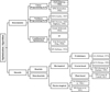 |
Fig. 1 Classification of optimization algorithms. |
2.1 Mathematical model
The TSP can be formulated as an integer linear programming problem, seeking to find a Hamiltonian cycle in a complete weighted graph. G = (V, E), representing the TSP. Here, V denotes the cities, V = {v1, v2, v3,…, vn}, and E represents the arcs. The distances are symmetric, meaning dij = dji where i and j are the distance between cities. The set of all Hamiltonian cycles H in G is given by: H = {(vi1, vi2, vi3,…,vin,vi1) | (vi1, vi2, vi3, …, vin)} is a permutation of (v1, v2, v3, …, vn.). The objective functions f1, f2, and f3 are focused on minimizing the total travel distance, travel time, and travel cost, respectively.
Objective function:
 (1)
(1)
 (2)
(2)
 (3)
(3)
 (4)
(4)
 (5)
(5)
 (6)
(6)
where tij denotes the travel time of arc (i, j), cij denotes the cost of arc (i, j), ui prevents sub-tours from city i, and xij is the decision variable. Here, w1, w2, and w3 represent the weighting factors assigned to each objective in the multi-objective optimization framework. Organizations can adjust these weights based on their specific performance priorities and optimization goals to reflect their preferences more accurately.
Subject to:
 (7)
(7)
 (8)
(8)
 (9)
(9)
 (10)
(10)
 (11)
(11)
 (12)
(12)
The objective function defined in equations (1), (2), and (3) aims to minimize the total distance, travel time, and travel cost, respectively. Equations (4), (5), and (6) define the multi-objective optimization by calculating the weighted sum of distance, time, and cost, with each objective assigned a corresponding weight. Equations (7) and (8) ensure that each city is visited exactly once and departed exactly once. Equation (9) prevents sub-tour formation, guaranteeing a single continuous loop that includes all cities. The binary variable xij in equation (10) indicates whether the path from city i to city j is included in the tour. In (11) and (12), the variable ui is used to enforce the subtour elimination constraints and is treated as a continuous variable.
2.2 Greedy algorithm
Greedy algorithms prioritize the most immediate outcome, producing locally optimal decisions at each step. It focuses without considering the overall context. The GrA chooses the most favourable edge at each step without considering the overall scenario Baidoo and Oppong [37]. Although GrA may not always ensure the most accurate solution, they frequently deliver satisfactory results, particularly when obtaining the highly precise solution is prohibitively expensive. Even with their focus on local optimality, greedy algorithms are capable of approximating global optima within acceptable time limits. Additionally, the choice of starting vertex in TSP affects the resulting Hamiltonian Cycle. The modified Greedy Algorithm can be explained as follows Mecler et al. [38]:
1 Data: A set of tourist city locations on Chattogram V, v ∈ Vand C is the cost.
2 Result: The shortest distance of location V.
3 Procedure GREEDY (v∘, C)
4 
5 
6 While |V| < |C| do
7 next position ←minimum distance (current position, c) , ∀ c ∈ C V
8 
9 
10 end while
end procedure
2.3 Brute-force algorithm
The brute force method involves solving a problem by testing every possible solution until the correct one is found. This method is also referred to as the Naive Approach. It is a programming strategy that eschews cutoffs to enhance performance, relying instead on absolute computational power to explore all options until a reliable solution is found. To get optimal results, this algorithm must try all the permutations of city routes one by one that exist until every possible route has been investigated. Brute force is recognized for producing the optimal solution for the TSP. This traditional algorithm evaluates all possible combinations of nodes, resulting in extended execution times for larger datasets, particularly those involving more than 20 cities. Despite its slow performance, it consistently delivers the nearest optimum solution for the TSP. The modified Brute force Algorithm can be explained as follows Ariyanti et al. [39]:
1 A set of co-ordinates points of cities in Chattogram represented by P (Xi, Yi).
2 
3 for i← 1 to n − 1do
4 for j ← i + 1to n do
5 
6 If d< d min then
7 
8 return index1, insex2
2.4 Branch and bound algorithm
The Branch and Bound (B&B) algorithm is a systematic approach to exploring the solution space, which is typically organized into a tree-like structure known as a state space tree that enumerates all possible solutions to a problem [40]. The B&B algorithm primarily consists of three components: branching, bounding, and pruning. Branching involves dividing the entire set of possible solutions into smaller, more manageable subsets. Bounding, also referred to as delimiting, is the process of determining the best-case (upper bound) and worst-case (lower bound) scenarios for each subset following the evaluation of their primary nodes. Pruning involves eliminating branches that no longer contribute to finding the optimal solution, specifically when the lower bound of the current optimal solution is lower than the lower bound of a branch, leading to its removal. This method systematically narrows the search field until a viable solution is discovered. Typically, the solution derived using the B&B method is the optimal solution Zhang et al. [40]. The modified Branch and Bound Algorithm can be explained as follows by Morrison et al. [12]:
1 A set of cities L = {V} and initialize v.
2 While L ≠ ∅ :
3 Select a subprogram S from L to explore
4 if a solution 
5 If S can't be pruned:
6 Partition S into S1, S2, S3, … , Sr
7 Insert S1, S2, S3, … , Sr into L
8 Remove S form L
10 Return v
2.5 Dynamic programming
Dynamic programming is an efficient method for computing recurrences by storing and reusing partial results. It is well-known that dynamic programming recursions can be framed as shortest-path problems in a layered network, where the nodes represent the states of the dynamic program. In Balas et al. [41], a technique was proposed for solving the TSP by associating it with a network G* = (V*, A* ). This network comprises (n+1) layers of nodes, each layer corresponding to a position in the tour. The home city appears at both the beginning and the end of the tour, serving as both the source node S and the sink node t. The structure of G* rates a one-to-one correspondence between tours in G that satisfy certain conditions (referred to as feasible tours) and (s − t) paths in G* Furthermore, optimal tours in G correspond to the shortest (s − t) paths in G* . The modified Dynamic Programming Algorithm can be explained as follows by Bouman et al. [22]:
Data: A set of tourist city locations on Chattogram V, an arbitrary location v ∈ V, and the cost function of the tour is c.
Result: A shortest-distance tour that covers all locations V only once.
1 Initialize DTSP with the value ∞ ;
2 Taking a table P to retain predecessor locations of the cities.
3 Initialize v as an arbitrary location in V;
4 for each w ∈ V do
5 
6 
7 for i = 2, … , |V| do
8 for S ⊆ Vwhere|S| = i do
9 for each w ∈ S do
10 for each u ∈ S do
11 
12 If z< DTSP (S, w) then ;
13 
14 
15 Return path obtained by backtracking over locations in P starting at P (V, v) ;
2.6 Nearest Neighborhood Algorithm
The NN algorithm is a heuristic used to solve the TSP by constructing a tour through an iterative selection of the closest unvisited city. Starting from an initial city, it adds the nearest unvisited city to the path until all cities are visited, then returns to the starting city. The NN algorithm is simple and fast, making it suitable for large datasets requiring quick solutions. However, it does not always produce the optimal solution and can yield suboptimal tours. Despite this, it serves as a useful baseline for comparing more advanced optimization techniques and can be refined further in hybrid approaches. The modified Genetic Algorithm can be explained as follows.
1 Input and Output: We input an n × n distance matrix D (dij, s) and an index s of the starting city. A list of paths of vertices containing the tour is obtained as an output.
2 Procedure Nearest Neighborhood Algorithm
3 Nearest Neighborhood D ([i = 1, … , n, j = 1, … , n] , s)
4 
5 Initialize the list Path with s
6 Visited[i]i ← true
7 
8 
9 Find the lowest element in row 𝑖 and unmarked column 𝑗
10 
11 
12 Add j to the end of the list path.
13 Add s to the end of the list path.
14 Return path
2.7 Genetic algorithm
The Genetic algorithm is an optimization technique that employs a stochastic method to randomly explore potential solutions for a given problem. By leveraging analogies from natural systems, these stochastic approaches generate promising solutions, offering higher efficiency compared to a purely random search. Each chromosome in the GA represents a potential solution, typically as a path through the cities in the TSP. The process begins with an initial random population and iteratively applies selection, crossover, and mutation to evolve the population toward an optimal solution. The GA continues until the population converges, yielding the shortest possible route through all cities. The modified Genetic Algorithm can be explained as follows George and Amudha [42]:
1 Procedure Genetic Algorithm ()
2 Initialization: Produce a random population of solutions(chromosomes)
3 For each individual iϵP:
4 Calculate the fitness(i):
5 Repeat
6 For i = 1to the number of the generations;
7 Select an operation randomly (crossover or mutation);
8 If crossover
9 Select two parents iaandib at random;
10 Produce an offspring ic = crossover (ia and ib) ;
11 Else if mutation:
12 Randomly select one chromosome I;
13 Produce an offspring ic = mutate (i) ;
14 End if;
15 Local seah (ic) ;
16 The fitness of the offspring ic is calculated;
17 If ic is better, then replace the worst chromosome with ic ;
17 Next i ;
18 Check termination = true;
19 End for
20 Return the fittest individual to P.
End procedure
2.8 Ant Colony Optimization
Ant Colony Optimization (ACO), originally introduced by Dorigo et al. [43], has proven to be an effective approach for solving the Traveling Salesman Problem (TSP), a classic combinatorial optimization challenge. In the TSP context, ACO simulates the pheromone-guided behavior of real ants to probabilistically construct paths that visit each city exactly once while minimizing the total travel cost. According to r50Nayyar and Singh [44], ACO's decentralized search mechanism, based on local pheromone information and iterative solution improvement, naturally extends to address multi-objective variants of TSP, where conflicting goals such as minimizing distance, time, and cost must be optimized simultaneously. By adjusting pheromone update rules and integrating multiple heuristic factors into the path construction process, ACO can balance trade-offs among objectives without relying on a single aggregated cost function. Nayyar and Singh's analysis further supports that adaptive versions of ACO, such as IACR, enhance performance by dynamically adjusting exploration and exploitation strategies, thereby producing diverse high-quality solutions for multi-objective optimization problems. The positive feedback and distributed learning inherent in ACO make it especially suited for multi-criteria decision-making scenarios like TSP, where robustness, flexibility, and convergence toward Pareto-optimal solutions are essential [44].The modified Ant Colony Optimization (ACO) Algorithm can be explained as follows by [44]:
1 Procedure of Ant Colony Optimization algorithm()
2 A TSP instance with cities C and distance function d(ci,cj) InitializePheromoneValues(τ)
3 Sbs ← NULL
4 while termination conditions not met do
5 Siter ← ϕ
6 for j = 1,…, nants do
7 S ← ConstructTour(τ)
8 if is a valid tour then
9 𝑠 ← LocalSearch(s) {optional}
10 if Cost (𝑠) < Cost (𝑠𝑏𝑠) or 𝑠𝑏𝑠 = NULL then
11 𝑠𝑏𝑠 ← s
12 end if
13 Siter ← Siter ∪ {s}
14 end if
15 end for
16 ApplyPheromoneUpdate(τ, Siter, 𝑠𝑏𝑠)
17 end while
18 Output: The best-so-far tour sbs
2.9 Particle Swarm Optimisation (PSO)
Particle Swarm Optimisation (PSO), inspired by the collective foraging behavior of birds and fish, has been effectively adapted to solve the Traveling Salesman Problem (TSP), a classic combinatorial optimization task. In PSO applied to TSP, each particle represents a candidate tour, a permutation of cities and updates its solution through a set of swap operations, which act as discrete analogs to velocity and position updates. As shown by Bilandi et al. [45], while PSO offers strong exploration capabilities in high-dimensional search spaces, it risks premature convergence to local optima in complex landscapes like TSP. To address this, multi-objective formulations of the TSP incorporate competing criteria such as minimizing distance, cost, and travel time simultaneously. In this setting, PSO can be extended by modifying velocity updates to consider multiple objectives, guiding particles toward Pareto-optimal fronts rather than a single global optimum. The hybridization techniques, such as integrating Simulated Annealing (SA) with PSO (hPSO-SA), further enhance the local search capabilities, balancing exploration and exploitation phases more effectively. This adaptability makes PSO a promising candidate for solving multi-objective TSPs, where trade-offs between various objectives must be dynamically managed during the optimization process [45]. The modified Particle Swarm Optimisation (PSO) algorithm can be expressed as follows by Bilandi et al. [45].
1 The distance between the city d(ci,cj) at maximun iteration MIiter with N cities
2 for i = 1 to N do
3 pi ←Randomly initialize a valid tour (a permutation of cities)
4 
5  then
then
6 
7 End if
8 Initialize velocity vi (velocity could be a set of swap operations)
9 end for
10 while t < MIitert do
11 
12 for i = 1 to N do
13 Update the velocity 𝑣𝑖 using swap sequences or edge exchanges
14 Apply the velocity vi to tour pi to generate a new tour
15  then
then
16 
17  then
then
18 
19 end if
20 end if
21 end for
22 end while
23 Output: The global best tour GObest
2.10 Simulated Annealing (SA)
Simulated Annealing (SA) is a stochastic metaheuristic algorithm inspired by the annealing process in metallurgy, and it has been widely applied to solving the Traveling Salesman Problem (TSP). In the context of TSP, as depicted in the provided pseudocode, SA begins with an initial valid tour and iteratively explores neighboring tours by introducing small changes, such as swapping the order of cities. Each candidate tour is accepted based on the Metropolis criterion: better solutions are always accepted, while worse solutions are accepted with a probability related to the current temperature, allowing the algorithm to escape local minima. A crucial aspect of the process is the setting of the initial temperature (T₀), which acts as an artificial control parameter manually set by the user to manage the randomness and acceptance of worse solutions in the early stages of the search.it does not depend on the cities or distance data. As the algorithm progresses, T₀ gradually decreases according to a cooling schedule, shifting the focus from exploration to exploitation. According to Kuznetsov et al. [46], SA's flexibility in adjusting parameters like T₀ and the cooling rate makes it particularly effective for multi-objective TSP problems, where multiple goals such as minimizing distance, balancing time, and reducing cost must be optimized simultaneously. This adaptability allows SA to approximate Pareto-optimal solutions rather than converge prematurely to a single suboptimal path, making it a powerful tool for complex combinatorial optimization challenges. The modified Simulated Annealing (SA) Algorithm is presented as followes of Kuznetsov et al. [46].
1 procedure simulated annealing for TSP returns a TOUR tour k
2 To, initial temperature
3 
4 
5 
6 
7 
8 
9 
10 end if
11 
12 end for
return tour k
end procedure
3 Tourist places
The current study comprehensively investigates eight tourist spots in the Chattogram division, including Chattogram, Bandorban, Rangamati, Khagrachari, Sajek, Cox's Bazer, Teknaf, and Saint Martin in Figure 2. The data for this study were collected using “Google Maps” and subsequently verified through personal travel. Three distinct data matrices are used here: distance, travel time, and traveller cost. In this study, the traveller is considered to begin and conclude his journey in Chattogram. These considerations result in an 8 × 8 city matrix which provides crucial information about the distance, time, and cost. Hence. A total of 40320 (=8!) possible routes are found. Consequently, it is quite impossible for a person to choose the most optimal travel route without using any computational tools. Inspired by this, the current study employs distinct algorithms and performs a comparison study to obtain optimal route solutions for the above-mentioned problem. Plan a trip to Chattogram that aims to visit a selection of its key tourist spots. The map below displays the locations of these attractions.
The TSP graph below illustrates cities as nodes, and the distances, times, or costs between them as edges are expressed in Figure 3. It also shows the possible route combinations between these cities. Each city has eight possible routes for entering or exiting. The combination always starts and ends the tour in Chattogram City.
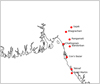 |
Fig. 2 Highlighted map of 8 tourist places in Chattogram division. |
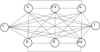 |
Fig. 3 Possible combination of routes. |
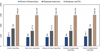 |
Fig. 4 Comparison of distance, time, and cost using different algorithms. |
4 Performance analysis
Each algorithm was executed ten times using the city matrix for three categories: distance, time, and cost are presented in Table 1. In this section, we investigate the results of the proposed optimization algorithms. It should be noted that all the code for the proposed algorithm was written in Python 3, and the experiments were conducted on a laptop equipped with an Intel(R) Core(TM) i5-7200U CPU @ 2.50GHz − 2.70 GHz and 8 GB of RAM with 64-bit operating system, x64-based processor.
The result of each algorithm is tabulated in Table 1. The optimal value from each problem and category is indicated in bold font. Each algorithm exhibits a unique pattern of computation time; the GrA is the fastest among them for the same data set but does not always provide the optimal solution in terms of distance or cost. The reason behind the quick response of the greedy algorithm is that it makes locally optimal decisions at each step without backtracking, significantly reducing computational complexity. This simple, iterative approach allows for fast execution, though it may not always yield the optimal solution. Based on the table, the algorithm demonstrating an average near-optimal solution for all categories is DP, followed by BF. B & B also shows better-quality results. The reason for better average results in the DP algorithm's efficacy may be attributed to its diversification mechanism (Breaks problems into overlapping subproblems, utilizes memorization or tabulation to store results), which excludes the undesired result and ensures a better performance.BF finds the optimal solution in terms of distance and cost, but it's less efficient in terms of execution time compared to the Greedy and NN algorithms. B&B matches the BF in solution quality but takes longer to execute. Although BF, B&B, and DP algorithms show the same result, they present different behaviour in terms of execution time. DP shows the optimal route in less execution time among them. Fast is like the greedy algorithm but less optimal in achieving the lowest distance and cost as depicted in the Figure 4.
The large problem requires extended computational time and impacts the quality of the solution's construction and accuracy. Figure 5 compares the average execution times of various deterministic optimization algorithms when applied to a specific problem, enabling a straightforward assessment of their computational speed. This analysis reveals that B&B exhibit considerably longer execution times of 0.04275 s, respectively, which are significantly longer than those recorded for the other algorithms evaluated (see Fig. 5). Conversely, the Greedy Algorithm is found to be the fastest, followed by NN, DP, and BF Algorithms, respectively. This comparison highlights the efficiency of these algorithms in solving a problem of a specific size, suggesting their appropriateness for applications where computational performance is prioritized.
The performance of the algorithms is detailed below.
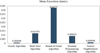 |
Fig. 5 Mean Execution time comparison. |
4.1 Stochastic algorithm
Figure 6 presents a comparative evaluation of four metaheuristic algorithms, genetic Algorithm (GA), Ant Colony Optimisation (ACO), Simulated Annealing (SA) and Particle Swarm Optimisation (PSO) across three performance metrics: total distance travelled, computational time, and overall cost. SA consistently outperforms the others, achieving the shortest tour (861.39 km), the shortest time to travel (1,571 min) and the smallest cost (2,910.28 Tk), thereby demonstrating superior convergence efficiency. GA and PSO exhibit nearly identical behaviour, each producing moderate tour lengths (886 km), runtimes (1,660 min) and costs (2,964.39 Tk). In contrast, ACO incurs the most tremendous expense in all three dimensions–longest path (1,016.8 km), highest travel time (1,873 min) and most significant cost (3,252.16 Tk) reflecting its intensive pheromone-update mechanism. These results highlight SA's advantageous balance of solution quality and computational overhead for the Traveling Salesman Problem in tourist location selection.
The bar graph compares the execution times of four popular optimization algorithms presented in Figure 7. The GA, ACO, SA, and PSO algorithms are applied to the Traveling Salesman Problem (TSP). Among these, ACO demonstrates the highest execution time, taking 3.623 seconds, highlighting its computationally intensive nature due to the need for multiple iterations and pheromone updates. In contrast, GA performs the fastest with an execution time of 0.04434 seconds, suggesting that it can find solutions more efficiently for the given problem instance. SA, with a time of 0.0153 seconds, also performs relatively well in terms of speed, being quicker than ACO but slower than GA. PSO, at 0.122 seconds, falls in between, striking a balance between exploration and exploitation. This comparison underscores the trade-off between solution quality and computational cost, where ACO, while effective, requires significantly more computational resources, whereas GA and SA provide faster solutions, making them more suitable for scenarios with strict time constraints. The results from this graph are crucial for selecting the most appropriate algorithm depending on the specific requirements of the TSP instance, such as speed or accuracy.
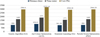 |
Fig. 6 Comparison of distance, time, and cost using different stochastic algorithms. |
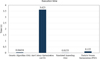 |
Fig. 7 Mean Execution time comparison of stocastic algorithm. |
4.2 Multi-objective optimisation
Figure 8 illustrates the multi-objective optimized values, aggregating distance, time, and cost metrics − achieved by nine algorithms, categorized into deterministic and stochastic approaches. Among the deterministic methods, the exhaustive and exact techniques, Brute Force (1,687.06), Branch and Bound (1,687.06) and Dynamic Programming (1,687.06), attain the lowest (best) optimized value. In contrast, the Greedy heuristic (1,775.72) and Nearest-Neighbourhood algorithm (1,793.26) yield higher values, reflecting suboptimal route choices. In the stochastic group, Simulated Annealing (1,688.94) closely approaches the exact optimum, while Genetic Algorithm and Particle Swarm Optimisation coincide at 1,741.72, and Ant Colony Optimisation performs least favourably at 1,944.27. These observations confirm that deterministic exact algorithms guarantee superior optimality at the expense of computational effort, whereas stochastic metaheuristics provide a spectrum of solution qualities with varying trade‑offs between optimality and algorithmic complexity. Based on these comparisons, the dynamic programming algorithm was selected as the optimal method for selecting tourist locations among the eight cities.
The dynamic programming algorithm completes in 0.008623 seconds, while marginally slower than the simplest heuristics (e.g., Nearest Neighbor at 0.00998 s and Branch and Bound at 0.00178 s) is still an order of magnitude faster than Brute Force (0.33142 s) and several orders faster than Ant Colony Optimization (3.623 s) is presented in Figure 9. This confirms that dynamic programming delivers exact optimality with negligible computational overhead, further supporting its practical viability for eight-city tourist-location selection.
The DP algorithm proves to be the most effective algorithm for solving the TSP, based on its superior performance across the key parameters of distance, travel time, cost, and execution time, as detailed in the Effectiveness Comparison of Algorithms section. According to Table 2, DP achieves optimal results with a distance of 886 km, travel time of 1661 minutes, and cost of 2964.399 Tk, yielding a multi-objective optimization value of 1742.02. Despite its slightly higher execution time of 0.008623 seconds, DP is still significantly more efficient than the B&B algorithm, which takes 3.623 seconds to execute, and BF, which takes 0.33142 seconds. Notably, DP provides the best balance between optimality and computational efficiency. While the GrA and NN algorithms are much faster, with execution times of 0.00564 seconds and 0.000998 seconds, respectively, their solutions are suboptimal, particularly in terms of distance and cost. In contrast, DP ensures that the solution is both optimal and efficient, making it the most effective for solving TSP in practical applications.
On the other hand, stochastic algorithms like GA, ACO, SA, and PSO, while delivering competitive performance in terms of solution quality, still fall short compared to DP. Specifically, ACO takes the longest execution time of 3.623 seconds but offers a higher multi-objective optimization value of 1944.27, though its long computational time makes it less efficient. GA, SA, and PSO have better execution times than ACO but still cannot match DP in terms of optimality. Thus, the DP algorithm remains the most effective algorithm, providing the best combination of optimal solution quality and execution time, making it the preferred choice for route optimization in tourism and business applications, where both accuracy and computational efficiency are critical.
The DP algorithm demonstrates the best results across the four parameters: distance, travel time, travel cost, and execution time, as shown in Table 2, followed by the BF and B&B algorithms. The computational time of the DP algorithm is 5 times faster than B&B and 1.4 times faster than BF, which provides the closest solution to DP. However, the DP algorithm is approximately 17 times slower than the quickest algorithm in this study. Thus, the optimal algorithms are determined by execution time, and the optimal routes for distance, travel time, and travel cost are presented in Figure 10. The cities are sequentially arranged as Chattogram, Rangamati, Bandorban, Sajek, Khagrachari, Cox's Bazar, Teknaf, and Saint Martin, represented by 1, 2, 3, 4, 5, 6, 7, and 8, respectively. The optimal route for distance is [1→ 4→ 5→ 2→ 3→ 6→ 7→ 8→ 1], indicating a traveller starts and ends their tour in Chattogram, as shown in Figure 10a. In Figure 10b, the path [1→ 3→ 6→ 7→ 8→ 5→ 4→ 2→ 1] represents the route for minimizing travel time. Reducing travel costs, a key aspect of the TSP, is achieved by the route [1→ 4→ 5→ 2→ 3→ 6→ 7→ 8→ 1]. Travelers can choose the route based on their specific needs.
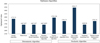 |
Fig. 8 Multi-objective optimized value of deterministic and stochastic algorithms. |
 |
Fig. 9 compares the execution times of deterministic and stochastic algorithms. |
Effectiveness comparison of the proposed algorithms.
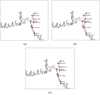 |
Fig. 10 The optimal routes are indicated by (a) for distance, (b) for travel time, and (c) for travel cost. |
5 Conclusion
Searching for the optimum routes in three city matrices using six optimization Deterministic algorithms: GrA, BF, B&B, DP, and NN and Stochastic algorithms: GA, ACO, SA, and PSO. The comparison encompasses computation time, statistical analysis of distance, travel time, travel cost, and execution time for each algorithm.
The Dynamic Programming (DP), Branch and Bound (B&B), and Brute Force (BF) algorithms resulted in identical optimal solutions in terms of shortest travel distance and minimum travel time, though each explored different routes.
Among these, DP is the most optimal algorithm, offering the shortest execution time while still maintaining the optimal solution. Despite B&B and BF yielding similar results, DP provides the best balance between computational efficiency and solution quality.
The Greedy Algorithm (GrA) was the fastest, but it failed to produce optimal solutions. On the other hand, the Genetic Algorithm (GA), although slower, did not outperform DP, B&B, or BF in terms of solution quality.
Ant Colony Optimization (ACO) achieved the best solution in terms of optimization, but it came with a high execution time, reflecting the computational cost of its iterative pheromone updates.
Simulated Annealing (SA) and Particle Swarm Optimization (PSO) showed a moderate execution time and were able to produce near-optimal solutions, making them versatile for a wider range of applications where speed and quality need to be balanced.
While stochastic algorithms generally excel in flexibility and scalability, ACO stands out for solution quality, but its long execution time may make it unsuitable for real-time applications with strict time constraints.
DP remains the most optimal choice for solving TSP, particularly for small to medium-sized problems where exact solutions are required. It stands out for its ability to provide optimal solutions while also minimizing execution time.
For larger problem sizes or cases where execution time is more critical, stochastic algorithms such as SA and PSO are more practical, offering near-optimal solutions with relatively faster runtimes compared to deterministic methods.
ACO, though delivering the highest quality solution, has a higher computational cost and may be less practical for real-time applications. However, its performance remains impressive for non-time-constrained scenarios.
The choice between deterministic and stochastic algorithms depends on the problem requirements, with DP being the most efficient for small to medium problems, and stochastic algorithms providing flexibility and faster approximations for larger or more dynamic environments. The trade-off between execution time and solution quality is a critical factor in selecting the appropriate algorithm for TSP.
Funding
This research did not receive any specific grant from funding agencies in the public, commercial, or nonprofit sectors.
Conflicts of interest
The authors declare that they have no known competing financial interests or personal relationships that could have appeared to influence the work reported in this paper.
Data availability statement
The data of this study are available from the corresponding author, upon reasonable request.
Author contribution statement
Md. Riad Hossen: Conceptualization, Data curation, Methodology, Validation, Investigation, Literature review, Python Programming, Visualization, Formal analysis, writing of review & editing and the original draft, Writing − review, and editing.
Hami Jafar Koushik: Conceptualization, Methodology, Validation, Investigation, Literature review, Formal analysis, Writing − review, and editing.
Mohammed Forhad Uddin: Supervision, Formal analysis, Writing − review, and editing.
Md. Atiqur Rahman: Model Validation, Investigation, Literature review, Formal analysis, Writing − review, and editing.
Md. Abdul Hye: Investigation, Literature review, Formal analysis, Writing − review, and editing.
References
- M.A.A. Hossain, Z.Y. Acar, Comparison of new and old optimization algorithms for traveling salesman problem on small, medium, and large-scale benchmark instances, Bitlis Eren Univ. J. Sci. 13, 216–231 (2024) [Google Scholar]
- D. Mecler, V. Abu-Marrul, R. Martinelli, A. Hoff, Iterated greedy algorithms for a complex parallel machine scheduling problem, Eur. J. Operat. Res. 300, 545–560 (2022) [Google Scholar]
- W. Li, L. Xia, Y. Huang, S. Mahmoodi, An ant colony optimization algorithm with adaptive greedy strategy to optimize path problems, J. Ambient Intell. Humanized Comput. 13, 1557–1571 (2021) [Google Scholar]
- J. Zhang, The logic and application of greedy algorithms, Appl. Comput. Eng. 82, 154–160 (2024) [Google Scholar]
- R. Zhang, Research on Enterprise Management Based on Greedy Algorithm, Atlantis Highlights in Engineering, 1134–1140 (2023) [Google Scholar]
- N.O.V. Eche, N.A.E. Okeyinka, N.I. Abdullah, N.A. Abdulrahman, Review of algorithms to solve travelling salesman problem, J. Sci. Innov. Technol. Res. 05 (2025) https://doi.org/10.70382/ajsitr.v7i9.019 [Google Scholar]
- S. Violina, Analysis of Brute Force and Branch & Bound Algorithms to solve the Traveling Salesperson Problem (TSP) (2021). https://turcomat.org/index.php/turkbilmat/article/view/3031 [Google Scholar]
- M.A. Fahroni, D. Pratiwi, A. Romadhoni, N.R. Syambas, Brute force modification algorithm for ring topology network optimization (2021). https://doi.org/10.1109/tssa52866.2021.9768247 [Google Scholar]
- S. Wahyuningsih, D.R. Sari, Study of the brand and bound algorithm performance on traveling salesman problem variants, Adv. Social Sci. Educ. Humanities Res. (2021) https://doi.org/10.2991/assehr.k.210508.066 [Google Scholar]
- E. Khalil, H. Dai, Y. Zhang, B. Dilkina, L. Song, Learning combinatorial optimization algorithms over graphs, Adv. Neural Inform. Process. Syst. 30 (2017) [Google Scholar]
- M. Dell'Amico, R. Montemanni, S. Novellani, Algorithms based on branch and bound for the flying sidekick traveling salesman problem, Omega 104, 102493 (2021) [CrossRef] [Google Scholar]
- D.R. Morrison, S.H. Jacobson, J.J. Sauppe, E.C. Sewell, Branch-and-bound algorithms: a survey of recent advances in searching, branching, and pruning, Discrete Optim. 19, 79–102 (2016) [Google Scholar]
- M. Gendreau, G. Laporte, F. Semet, Branch and price for the stochastic traveling salesman problem with time windows, Transport. Sci. 57, 656–672 (2023) [Google Scholar]
- S. Poikonen, B.L. Golden, E. Wasil, A branch-and-bound approach to the traveling salesman problem with a drone, Informs J. Comput. 31, 335–346 (2019) [Google Scholar]
- S. Dhanasekar, S. Dash, N. Uthaman, A branch and bound algorithm to solve travelling salesman problem (TSP) with uncertain parameters, Math. Stat. 10, 358–365 (2022) [Google Scholar]
- B. Dimitrijević, R. Jovanović, T. Burić, D. Teodorović, G. Ćirović, A comprehensive survey on the generalized traveling salesman problem, Eur. J. Operat. Res. 305, 409–428 (2023) [Google Scholar]
- N.S.M. Mussafi, Distribution route optimization of Zakat Al-Fitr based on the branch-and-bound algorithm, Int. J. Modern Trends Technol. Sci. 66, 528–533 (2023) [Google Scholar]
- S.-W. Lin, S. Guo, W.-J. Wu, Applying the simulated annealing algorithm to the set orienteering problem with mandatory visits, Mathematics 12, 3089 (2024) [Google Scholar]
- E. Baidoo, S.O. Oppong, Solving the TSP using traditional computing approach, Int. J. Comput. Appl. 152, 13–19 (2016) [Google Scholar]
- I. Ariyanti, M.A. Ganiardi, U. Oktari, Mobile application searching of the shortest route on delivery order of CV. Alfa Fresh with brute force algorithm, Logic/Logic: Jurnal Rancang Bangun Dan Teknologi 19, 120 (2019) [Google Scholar]
- G. Lera-Romero, J.J. Miranda-Bront, F.J. Soulignac, Dynamic programming for the time-dependent traveling salesman problem with time windows, INFORMS J. Comput. 34, 3292–3308 (2022) [Google Scholar]
- P. Bouman, N. Agatz, M. Schmidt, Dynamic programming approaches for the traveling salesman problem with drone, Networks 72, 528–542 (2018) [CrossRef] [MathSciNet] [Google Scholar]
- C. Malandraki, R.B. Dial, A restricted dynamic programming heuristic algorithm for the time dependent traveling salesman problem, Eur. J. Operat. Res. 90, 45–55 (1996) [Google Scholar]
- M.Z. Rahman, S. Sheikh, A.Z.M.T. Islam, M. Rahman, Improvement of the nearest neighbor heuristic search algorithm for traveling salesman problem, J. Eng. Adv. 19–26 (2024) [Google Scholar]
- E.O. Asani, A.E. Okeyinka, A.A. Adebiyi, A Construction Tour Technique For Solving The Travelling Salesman Problem Based On Convex Hull And Nearest Neighbour Heuristics. 0 International Conference in Mathematics, Computer Engineering and Computer Science (2020). https://doi.org/10.1109/icmcecs47690.2020.240847 [Google Scholar]
- T. George, T. Amudha, Genetic algorithm based multi-objective optimization framework to solve traveling salesman problem. In Algorithms for intelligent systems (2020) pp. 141–151 [Google Scholar]
- M. Dorigo, V. Maniezzo, A. Colorni, Ant system: optimization by a colony of cooperating agents, IEEE Trans. Syst. Man Cybern. Part B (Cybernetics) 26, 29–41 (1996) [Google Scholar]
- Y. Deng, Y. Liu, D. Zhou, An improved genetic algorithm with initial population strategy for symmetric TSP, Math. Probl. Eng. 2015, 1–6 (2015) [Google Scholar]
- S. Prayudani, A. Hizriadi, E.B. Nababan, S. Suwilo, Analysis effect of tournament selection on genetic algorithm performance in Traveling Salesman Problem (TSP), J. Phys. Conf. Ser. 1566, 012131 (2020) [Google Scholar]
- T. Kowalski, A review of the applications of genetic algorithms to forecasting commodity prices, Economies 9, 6 (2021) [Google Scholar]
- D. Yang, Z. Yu, H. Yuan, Y. Cui, An improved genetic algorithm and its application in neural network adversarial attack, PLOS ONE 16, e0251234 (2021) [Google Scholar]
- J. Zheng, J. Zhong, M. Chen, K. He, A reinforced hybrid genetic algorithm for the traveling salesman problem, Comput. Operat. Res. 157, 106249 (2023b) [Google Scholar]
- D. Shan, S. Zhang, X. Wang, P. Zhang, Path-planning strategy: adaptive ant colony optimization combined with an enhanced dynamic window approach, Electronics 13, 825 (2024) [Google Scholar]
- G. Dantzig, R. Fulkerson, S. Johnson, Solution of a large-scale traveling-salesman problem, J. Oper. Res. Soc. Am. 2, 393–410 (1954) [Google Scholar]
- K. Tang, C. Meng, Particle swarm optimization algorithm using velocity pausing and adaptive strategy, Symmetry 16, 661 (2024) [Google Scholar]
- W. Kool, H. Van Hoof, J. Gromicho, M. Welling, Deep policy dynamic programming for vehicle routing problems, In Lecture notes in computer science (2022) (pp. 190–213) [Google Scholar]
- W. Li, L. Xia, Y. Huang, S. Mahmoodi, An ant colony optimization algorithm with adaptive greedy strategy to optimize path problems, J. Ambient Intell. Humanized Comput. 13, 1557–1571 (2021) [Google Scholar]
- A. Mingozzi, L. Bianco, S. Ricciardelli, Dynamic programming strategies for the traveling salesman problem with time window and precedence constraints, Operat. Res. 45, 365–377 (1997) [Google Scholar]
- C.S. Chauhan, R.K. Gupta, K. Pathak, Survey of methods of solving TSP along with its implementation using dynamic programming approach, Int. J. Computer Appl. 52, 12–19 (2012) [Google Scholar]
- J. Zhang, Comparison of various algorithms based on TSP solving, J. Phys. Conf. Ser. 2083, 032007 (2021) [Google Scholar]
- E. Balas, New Classes of Efficiently Solvable Generalized Traveling Salesman Problems,” MSRR No. 615, GSIA, Carnegie Mellon University, 1996 [Google Scholar]
- R.K. Halder, M.N. Uddin, M.A. Uddin, S. Aryal, A. Khraisat, Enhancing K-nearest neighbor algorithm: a comprehensive review and performance analysis of modifications, J. Big Data 11, (2024) Article 113 [Google Scholar]
- T. Xie, L. Chen, B. Yi, S. Li, Z. Leng, X. Gan, Z. Mei, Application of the improved K-nearest neighbor-based multi-model ensemble method for runoff prediction, Water 16, 69 (2024) [Google Scholar]
- A. Nayyar, R. Singh, Performance analysis of ACO based routing Protocols- EMCBR, ANTChain, IACR, ACO-EAMRA for Wireless Sensor Networks (WSNs), Br. J. Math. Comput. Sci. 20, 1–18 (2017) [Google Scholar]
- N. Bilandi, H.K. Verma, R. Dhir, hPSO-SA: hybrid particle swarm optimization-simulated annealing algorithm for relay node selection in wireless body area networks, Appl. Intell. 51, 1410–1438 (2020) [Google Scholar]
- A. Kuznetsov, L. Wieclaw, N. Poluyanenko, L. Hamera, S. Kandiy, Y. Lohachova, Optimization of a simulated annealing algorithm for S-Boxes generating, Sensors 22, 6073 (2022) [Google Scholar]
Cite this article as: Md. Riad Hossen, Hami Jafar Koushik, Mohammed Forhad Uddin, Md. Atiqur Rahman, Md. Abdul Hye, Optimal algorithm of the traveling salesman problem for tourist location selection, Int. J. Simul. Multidisci. Des. Optim. 16, 11 (2025), https://doi.org/10.1051/smdo/2025011
All Tables
All Figures
|
Fig. 1 Classification of optimization algorithms. |
| In the text | |
|
Fig. 2 Highlighted map of 8 tourist places in Chattogram division. |
| In the text | |
|
Fig. 3 Possible combination of routes. |
| In the text | |
|
Fig. 4 Comparison of distance, time, and cost using different algorithms. |
| In the text | |
|
Fig. 5 Mean Execution time comparison. |
| In the text | |
|
Fig. 6 Comparison of distance, time, and cost using different stochastic algorithms. |
| In the text | |
|
Fig. 7 Mean Execution time comparison of stocastic algorithm. |
| In the text | |
|
Fig. 8 Multi-objective optimized value of deterministic and stochastic algorithms. |
| In the text | |
|
Fig. 9 compares the execution times of deterministic and stochastic algorithms. |
| In the text | |
|
Fig. 10 The optimal routes are indicated by (a) for distance, (b) for travel time, and (c) for travel cost. |
| In the text | |
Current usage metrics show cumulative count of Article Views (full-text article views including HTML views, PDF and ePub downloads, according to the available data) and Abstracts Views on Vision4Press platform.
Data correspond to usage on the plateform after 2015. The current usage metrics is available 48-96 hours after online publication and is updated daily on week days.
Initial download of the metrics may take a while.