")
")
| Issue |
Int. J. Simul. Multidisci. Des. Optim.
Volume 9, 2018
|
|
|---|---|---|
| Article Number | A2 | |
| Number of page(s) | 6 | |
| DOI | https://doi.org/10.1051/smdo/2017009 | |
| Published online | 16 March 2018 | |
Research Article
New approach for getting better accuracy with mesh dependent material properties
Institute of Industry Technology, Guangzhou & Chinese Academy of Sciences,
1121 Haibin Road,
511458
Guangzhou,
Guangdong, PR China
* e-mail: This email address is being protected from spambots. You need JavaScript enabled to view it.
Received:
27
November
2017
Accepted:
20
December
2017
Abstract
Based on the relationship between finite element (FE) solution and mesh size, a new approach based on mesh depending on the material properties is proposed to make the finite element analysis results more efficient and more close to the optimal solution. This optimal solution is often evaluated either by experiment or by finite element method (FEM). At the opposite of the accuracy obtained by sensitivities analysis of the FEM which requires time-consuming, our approach allows getting the optimal meshing based on the material properties.
Key words: Parameters identification / mesh dependency on material properties / finite element mesh
© Q.-P. Zhou and H. Ding, published by EDP Sciences, 2018
 This is an Open Access article distributed under the terms of the Creative Commons Attribution License (http://creativecommons.org/licenses/by/4.0), which permits unrestricted use, distribution, and reproduction in any medium, provided the original work is properly cited.
1 Introduction
The solving process in finite element method (FEM) includes four main steps: first step, is to discrete the physical model. Second step, is to determine the governing equations and their boundary conditions. Third step, is to give the finite element (FE) equations of discrete elements. Finally, to solve the FE equations by a joint solution. Meshing is a critical step in FEM [1–3]. It affects directly the accuracy of analysis results. The choice of mesh size in FEM is the eternal question for numerical simulation [4,5]. The accuracy of the meshing size depends on the geometries of the domain, the materials properties, the element types and the loading. Theoretically, for FEM under certain conditions, the accuracy of the mesh is more precise when it's size is quite small. However, such as small size lead to high computation cost. Concretely, one should follow the algorithm below to reach the optimal precision ε:
-
Start with initial mesh size equal to h1;
-
form Kh1 (stiffness matrix) and Fh1 (discrete loads) we solve Kh1. Uh1 = Fh1;
-
Choose a new mesh size h2 that respect h2 < h1;
-
Then, form Kh2 and Fh2 we solve again Kh2. Uh2 = Fh2;
-
If
 then Stop, Uh2 is the final solution, Otherwise, h1 = h2;
 -
Return to Step 1.
However, the above approach cost a lot in term of computation time. In practical, the mesh size is often chosen by experience [6–9]. On the other hand, the material is often homogenised when performing FE analysis at a macroscopic scale. The mesh size cannot be infinitely reduced. Indeed, we can mesh the local structure, but in this case, we face the time computing and also a cross-size simulation. When we select the mesh size for FE simulation, there must be some error in the FE solution and in the solution of the differential equation. In general, this error is monotonous to the mesh size. For the FEM using the displacement method, the stiffness of the finite element model increases with the increase of the mesh size under certain conditions [10–13]. In this article, we propose a new approach to identify the mesh dependency on material properties to solve this problem.
2 Relationship between FEM accuracy and mesh size
In this section, we underline above all through an basic example of cantilever beam the relation between the meshing size and the response of the structure.
2.1 Example: the cantilever beam subjected to uniform load
As discribed in Figure 1, a representative cantilever beam subjected to uniform load is discussed in this section (Fig. 2). The beam section is I50a, where y-axial moment of inertia is Iy = 1120 cm4. The length of the beam is L = 2000 mm. The material properties of the beam are: Young's modulus E = 210 Gpa and the Poisson's ratio μ = 0.3. The bean is under uniform loading with the following density per length unit q = 10 N/mm.
The theoretical equation for deflection curve is  . At the end of the free edge, it is equal to
  . Once, we consider the numerical values, WB = 8.5034 mm.
The length of the beam, the cross-sectional dimension, the load and the material properties remain unchanged, changing the mesh size h, we obtain in Table 1 the displacement of the cantilever beam WB(h) at different mesh size.
As shown in the above table and figure, the displacement in function of the mesh size WB(h) converges to the theoretical solution WB when the mesh size is small enough (h converges to zero).
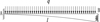 |
Fig. 1 Cantilever beam subjected to uniform load. |
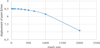 |
Fig. 2 Displacement of the cantilever beam at different mesh size. |
Displacement of the cantilever beam at different mesh size.
2.2 Relation between finite element solution and mesh size
Using the minimum potential energy principle, we obtain the following static equation
 (1)
where, Kh is the FE stiffness matrix that dependent on Young's modulus, the Poisson's ratio. Uh is the nodal displacement and Fh is the equivalent nodal load.
(1)
where, Kh is the FE stiffness matrix that dependent on Young's modulus, the Poisson's ratio. Uh is the nodal displacement and Fh is the equivalent nodal load.
The elastic deformation energy of the approximate solution of the displacement obtained by using the minimum potential energy principle is the lower bound of the exact solution deformation energy (the approximate displacement field is smaller than the exact solution). As we know the finite element solution is:
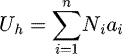 (2)
where, Ni and ai are respectively the shape interpolation function and the weight parameter for each i.
(2)
where, Ni and ai are respectively the shape interpolation function and the weight parameter for each i.
When n is big, there are more parameters to be determined, the accuracy of the finite element solution is higher. When n tends to infinity, the approximate solution approaches the exact solution. So the displacement Uh converges to the exact solution U0 when the mesh size tends to zero (see Fig. 3).
 |
Fig. 3 Displacement of the domain at different mesh size. |
3 Mesh dependent material properties
Material properties are usually obtained by physical tests. For example, the Young's modular E can be obtained from the one dimension tensile test (Fig. 4). The values will depend only on the measurement of stress and strain.
However, the measurements of stress and strain are not the objective. They depend on which kind of measurements you used: sample type, measurements of the geometry, loads and/or evaluation methods of stress and strain. Using FEM as a rule to evaluate σ and ε or U etc, to obtain E and μ. Given element size h, element type, sample geometry etc, form Kh which is depend on E and μ, solve
 (3)
(3)
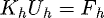
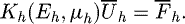
We obtain mesh dependent evaluations:
 (4)
where, Kh(Eh, μh) is the stiffness matrix when the mesh size is h, Eh is the Young's modulus and μh is the Poisson's radio,
(4)
where, Kh(Eh, μh) is the stiffness matrix when the mesh size is h, Eh is the Young's modulus and μh is the Poisson's radio,  is the nodal displacement when the mesh size is h;
  is the load when the mesh size is h.
  and
and  can be obtained by simulation or experiment.
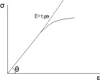 |
Fig. 4 Stress-strain curve. |
4 Numerical examples
In this section, some numerical examples are calculated to illustrate the proposed method. First, the optimal solutions to meet a certain accuracy of a typical one dimension tensile model and a shear dominant model are obtained. Then, based on the solutions, we obtain the related mesh that depends on material parameters Eh and μh with a certain accuracy. We consider for this example a cubic structure structure subjected to uniform loads. The mesh scale k is evaluated as:
 (5)
where h is the mesh size, lo is the minimum characteristic dimension of concern.
(5)
where h is the mesh size, lo is the minimum characteristic dimension of concern.
4.1 Example of accuracy for a cuboid under different loading case
In the following, we will present 3 cases of loading for better understanding.
4.1.1 Case 1: Tension loading
As displayed in Figure 5, the simulation model is a cubic structure 5 cm × 5 cm × 10 cm subjected to one dimension tensile load 200 Mpa on a 5 cm × 5 cm section. The material properties of the cubic structure are Young's modulus E = 210 Gpa and the Poisson's ratio μ = 0.3.
We choose the accuracy of the solution is ε = 10−3. Than, we reduce gradually the mesh size from 50 mm to 3.1 mm in order converge to the optimal value ε that we consider after as a reference value. The error of the solution before and after encryption meet than the parameter ε.
In Table 2 and Figure 6, we obtain the following displacement Ut* = 9.37779 × 10⁻² mm at the smallest value of ϵ that corresponds a mesh scale equal to 0.0625.
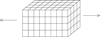 |
Fig. 5 One dimension tensile model. |
Elongation of the cubic structure at different mesh scale.
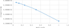 |
Fig. 6 Elongation of the cubic structure at different mesh scale. |
4.1.2 Case 2: Shearing loading
As displayed in Figure 7, the simulation model is a cubic structure 5 cm × 5 cm × 10 cm subjected to shear force 100 Mpa. The material properties remain the same.
We choose the accuracy of the solution ε equal to 3 × 10⁻³. As the previous case, we reduce the mesh size from 50 mm to 1.5 mm to reach the optimal ε (that we consider as a real or optimal solution).
Table 3 and Figure 8 show that the solution related to optimal ε gives Us* = 8.91528 × 10⁻¹ mm with a corresponding mesh scale equal to 0.03125.
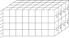 |
Fig. 7 Shear loading of the cubic structure. |
Displacement of the cubic structure at different mesh scale.
 |
Fig. 8 the displacement of the cubic structure at different mesh scale. |
4.1.3 Case 3: Mesh dependent material properties
Based on the previous target solutions with a certain accuracy, we obtain the mesh dependent material parameters Eh and μh. First we identify the Eh then we identify μh.
4.1.3.1 Identification of Eh
As the domain, the load and the Poisson's ratio remain unchanged (see Fig. 5), we change the mesh size value h to solve the following equality:

The material parameter Eh is identified afterward as described in Table 4 and in Figure 9.
Identified Young's modulus at different mesh scale.
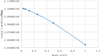 |
Fig. 9 Identified Young's modulus at different mesh scale. |
4.1.3.2 Identification of μh
As the domain, the load remain unchanged (see Fig. 7), and using the identified Young's modulus Eh we obtained above we change the mesh size h to solve the following equation to get parameter μh:

4.1.3.3 Application of the mesh dependency material properties
When we use the given mesh size to solve the real application (Fig. 10), we should introduce mesh dependent material properties Eh and μh (Tab. 5) to form the stiffness matrix Kh(Eh, μh). As displayed in Figure 11, the cubic structure 5 cm × 5 cm × 10 cm is subjected to uniform loading with the following density equal to 50 Mpa.
As the domain and the load remain unchanged during EF analysis, the comparison of the cases results 1–3 with different mesh size h are shown below : Case 1 in Table 6, case 2 in Table 7 and case 3 (using the identified parameters Young's modulus Eh and the identified Poisson's ratio μh) in Table 8.
As we can see in Figure 12 after Young's modulus and Poisson's ratio correction, the mesh size can increase almost two levels to reach the same accuracy.
 |
Fig. 10 Identified Poisson's ratio at different mesh scale. |
Identified Poisson's ratio at different mesh scale.
 |
Fig. 11 Cubic structure under uniform loading. |
Displacement of the cubic structure at different mesh scale (Case 1).
Displacement of the cubic structure at different mesh scale (Case 2).
Displacement of the cubic structure at different mesh scale (Case 3).
 |
Fig. 12 Displacement of the cubic structure at different mesh scale. |
5 Conclusion
In the finite element analysis, the structural response is related to the mesh size under certain conditions, the solution of FE analysis is increase uniformly to converge to the exact solution. However, with the discontinuity of the materials and non uniform shape such as composite and pore materials, the mesh size cannot be too small, otherwise, it will cause imprecise. The introduction of mesh dependent material properties correction results in more accurate results. Moreover, the Young's modulus and the Poisson's ratio correction together gave better accuracy than with only modulus correction. Finally, the correction is more efficient for coarse mesh than for fine mesh. This interval is also what we need to improve most.
References
- Ho-Le K. 1988. Finite element mesh generation methods: a review and classification. Computer-Aided Design, 20, 27–38. [CrossRef] [Google Scholar]
- Hughes TJR, Cottrell JA, Bazilevs Y. 2005. Isogeometric analysis: CAD, finite elements, NURBS, exact geometry and mesh refinement. Computer Methods in Applied Mechanics and Engineering, 194, 4135–4195. [Google Scholar]
- Van der VJJW, Van der VH. 2002. Space-time discontinuous galerkin finite element method with dynamic grid motion for inviscid compressible flows: I. General formulation. Journal of Computational Physics, 182, 546–585. [CrossRef] [Google Scholar]
- Jiang ZR, Duan PF, Guo XL, Ding H. 2010. Improvement of FEM's dynamic property. Applied Mathematics and Mechanics, 31, 1337–1346. [CrossRef] [Google Scholar]
- Gomes S, Bluntzer JB, Bassir D. 2008. Optimization of parametric CAD models for functional product design using PLM system. International Journal for Simulation and Multidisciplinary Design Optimization, 2, 83–90. [Google Scholar]
- Liszka T, Orkisz J. 1980. The finite difference method at arbitrary irregular grids and its application in applied mechanics. Computers & Structures, 11, 83–95. [CrossRef] [MathSciNet] [Google Scholar]
- Ollivier-Gooch C, Van Altena M. 2002. A high-order-accurate unstructured mesh finite-volume scheme for the advection-diffusion equation. Journal of Computational Physics, 181, 729–752. [CrossRef] [Google Scholar]
- Bassi F, Rebay S. 1997. High-order accurate discontinuous finite element solution of the 2D Euler equations. Journal of Computational Physics, 138, 251–285. [NASA ADS] [CrossRef] [MathSciNet] [Google Scholar]
- Zhang WH, Domaszewski M, Bassir D. 1999. Developments of sizing sensitivity analysis with ABAQUS code. Journal of Structural Optimization, 17, 219–225. [CrossRef] [Google Scholar]
- Zhu JH, Zhang WH, Xia L, Zhang Q, Bassir D. 2012. Optimal packing configuration design with finite-circle method. Journal of Intelligent and Robotic Systems, 67, 185–199. [CrossRef] [Google Scholar]
- Guessasma S, Bassir D. 2010. Optimization of elasticity parameters of cellular solids subject to structural anisotropy. Acta Materialia, 58, 716–725. [Google Scholar]
- Guessasma S, Bassir D, Hedjazi L. 2015. Influence of interphase properties on the effective behaviour of a starch-hemp composite. Materials & Design, 65, 1053–1063. [Google Scholar]
- Ding H, Zheng ZM, Xu SZ. 1990. A new approach to inverse problems of wave equations. Journal of Applied Mathematics and Mechanics, 11, 1113–1117. [CrossRef] [Google Scholar]
Cite this article as: Qiu-Ping Zhou, Hua Ding, New approach for getting better accuracy with mesh dependent material properties, Int. J. Simul. Multidisci. Des. Optim. 9, A2 (2018)
All Tables
All Figures
|
Fig. 1 Cantilever beam subjected to uniform load. |
| In the text | |
|
Fig. 2 Displacement of the cantilever beam at different mesh size. |
| In the text | |
|
Fig. 3 Displacement of the domain at different mesh size. |
| In the text | |
|
Fig. 4 Stress-strain curve. |
| In the text | |
|
Fig. 5 One dimension tensile model. |
| In the text | |
|
Fig. 6 Elongation of the cubic structure at different mesh scale. |
| In the text | |
|
Fig. 7 Shear loading of the cubic structure. |
| In the text | |
|
Fig. 8 the displacement of the cubic structure at different mesh scale. |
| In the text | |
|
Fig. 9 Identified Young's modulus at different mesh scale. |
| In the text | |
|
Fig. 10 Identified Poisson's ratio at different mesh scale. |
| In the text | |
|
Fig. 11 Cubic structure under uniform loading. |
| In the text | |
|
Fig. 12 Displacement of the cubic structure at different mesh scale. |
| In the text | |
Current usage metrics show cumulative count of Article Views (full-text article views including HTML views, PDF and ePub downloads, according to the available data) and Abstracts Views on Vision4Press platform.
Data correspond to usage on the plateform after 2015. The current usage metrics is available 48-96 hours after online publication and is updated daily on week days.
Initial download of the metrics may take a while.