")
")
| Issue |
Int. J. Simul. Multidisci. Des. Optim.
Volume 17, 2026
Multi-modal Information Learning and Analytics on Cross-Media Data Integration
|
|
|---|---|---|
| Article Number | 10 | |
| Number of page(s) | 15 | |
| DOI | https://doi.org/10.1051/smdo/2026005 | |
| Published online | 06 April 2026 | |
Research article
Landscape 3D visual perception simulation and path planning optimization algorithms based on deep learning
1
College of Fashion and Art Design, Gongqing College of Nanchang University, Jiujiang 332020, Jiangxi, PR China
2
College of Humanities, Gongqing College of Nanchang University, Jiujiang 332020, Jiangxi, PR China
3
College of Creative Arts, Universiti Teknologi MARA (UiTM), Shah Alam, Malaysia
* e-mail: This email address is being protected from spambots. You need JavaScript enabled to view it.
Received:
26
September
2025
Accepted:
31
December
2025
Abstract
Landscape environments present substantial difficulties for autonomous systems because of issues like vegetation occlusion, rolling terrain, varying light levels, and confusing textures that hinder accurate 3D perception and lead path planners to settle upon local optima or to run slowly. To attack this problem, this paper drinks a stride towards proposing the Landscape Perception-Planning Framework (LPPF), an end-to-end lightweight architecture capable of optimizing perception and planning jointly. LPPF includes a MobileNetV3–Swin Transformer architecture integrated to provide robust monocular depth estimation, construction of StyleGAN2-ADA generated synthetic 3D point clouds in multiple weather conditions for the purposes of generalization, and Proximal Policy Optimization (PPO) planner that dynamically adjusts depth confidence into a cost map for error-aware navigation. LPPF is evaluated using 10,000 synthetic LiDAR frames and 500 real LiDAR frames, achieving an overall score of 0.93, an improvement of 19.2% over DPT using the LPPF framework to process under a 50 ms real-time constraint on an embedded platform. By applying channel pruning and INT8 quantization, the model reduces parameters by 85.2% and increases inference by a factor of 3.21 indicating strong accuracy, robustness, and efficiency for intelligent navigation in complex, resource-constrained landscape environments.
Key words: Deep learning / 3D visual perception / path planning / lightweight framework / landscape environment
© F. Chen et al., Published by EDP Sciences, 2026
 This is an Open Access article distributed under the terms of the Creative Commons Attribution License (https://creativecommons.org/licenses/by/4.0), which permits unrestricted use, distribution, and reproduction in any medium, provided the original work is properly cited.
1 Introduction
As intelligent navigation systems are increasingly applied in urban inspections, ecological monitoring, and more, the need for the system to be adaptable to complex landscapes is quickly coming into focus. Typical landscapes (nature reserves, mountain trails, etc.), can present extreme video hoods including dense vegetation occlusion, rapid terrain changes, fluctuations in natural light, continual changes in weather, and considerable variation in materials. Each of these embodiments co-exist with other embodiments and have negative effects on visual perception and ultimately path planning. As an example, vegetation occlusion creates depth estimation blur, terrain changes create a polyhedral experience with an extreme geometric distortion, light changes create lessability in texture recognition, and changes in the reflective nature of materials removes the ability to see semantics and geometric boundaries. In landscape architecture, each of these visual systems challenges require some degree of solution. In particular, the challenging 3D visual weather in the autonomous path planning systems is especially challengeable along multiple dimensions of accuracy, robustness, and real-time performance [1–3]. The core research gap lies in the inadequate integration of perception and planning modules under strict real-time constraints, particularly for resource-constrained platforms operating in dynamic landscape environments. Most current studies will tend to apply a stepwise processing approach whereby 3D reconstruction occurs first with high accuracy, then path planning is completed on the basis of the reconstructed results. This leads to an irreconcilable conflict between the processing overhead for the perception module, requiring a large amount of computational resources and time, and a need for rapid responses in real time for path planning [4,5]. This imbalance between precision and latency severely restricts the actual deployment capability of the system in complex landscape environments, and fundamental optimization at the algorithm architecture level is required.
Existing research has shown a phased evolution in addressing this contradiction, but all paradigms have structural limitations. For example, the energy-optimized path planning method proposed by Ma B et al., which integrated land cover and terrain digital models, achieved energy efficiency improvement of three-dimensional tracks in complex field scenes [6]. The road footprint extraction method proposed by Ma H et al., which integrated PointNet++ and morphological post-processing, achieved high-precision segmentation of road areas from sparse LiDAR point clouds. However, it relied on high-cost airborne scanning data and output static maps. It was not suitable for real-time monocular vision input or dynamic path replanning requirements, and was difficult to embed into end-to-end navigation systems [7]. While existing studies focus on isolated perception or planning tasks, they neglect the synergistic optimization of both modules under real-time constraints, leading to suboptimal performance in dynamic landscapes. Similarly, the method proposed by Bai Z et al., which combined binocular vision simulation with semantic image segmentation, achieved a quantitative perceptual evaluation of visual elements of road landscapes. However, it focused on static aesthetic evaluation and did not extend to dynamic navigation decision-making or path optimization. It also lacked a systematic connection with autonomous obstacle avoidance and real-time trajectory generation of robots [8].
With the rise of deep learning, the second generation of methods attempted to use convolutional neural networks or visual transformers to enhance perception modules, such as monocular depth estimation or semantic segmentation, and to combine them with improved local obstacle avoidance algorithms. Arampatzakis V et al. comprehensively reviewed monocular depth estimation algorithms but did not address integration with path planning or lightweight deployment impacts on navigation latency [9]. Xu H et al.'s MFFP Net achieved high-precision building boundary segmentation but focused on static tasks without depth output or path planning integration, limiting robot navigation capability [10]. Tahir et al. reviewed adverse weather target detection and analyzed perception bottlenecks but did not link perception outputs to path planning or consider end-to-end latency and robustness [11]. Cao Y's VR-generated 3D art landscape simulation offered immersive visualization, but they concentrated on static aesthetics and lacked autonomous perception or path planning [12]. Półrolniczak M assessed perception through humans' changing landscape preferences relative to weather and seasonal changes but did not integrate visible robot perception or associated navigation decision-making [13]. Li Z et al.'s multi-teacher knowledge distillation framework improved 3D detection accuracy and inter-vehicle communication efficiency for multi-vehicle scenarios, but it concentrated specifically on detection components and ignored path planning integration or analysis of latency-robustness [14]. These efforts separate perception and planning to the detriment of robust generalization and enduring computation costs in dynamic landscapes.
The primary challenges include ambiguity in depth estimation when occluded by vegetation, limited generalization to extreme weather events, and brain template-to-action planning estimation accuracy and latency in planning response. Suanpang P's algorithm for D-Star-based drone autonomous navigation directly improved replanning efficiency, but only worked with pre-built maps, had no real-time perception and was limited in response to spontaneous obstacles [15]. Wu B used a hybrid A*-DWA algorithm for energy efficiency, but it also did not process dynamic obstacles [16]. Zhou Y used a biologically-inspired multi-robot-planning algorithm to navigate through dynamic mapped environments, yet it was limited to idealized sensors without visual percepts to prevent dynamic uncertainty related to weather obstacles or occlusion [17]. Lee D.H.'s end-to-end lane detection framework was not designed for lightweight and latency-constrained applications, resulting in inconsistent training and reduced generalization [18]. Liu C.'s UAV-based road inspection system required manual activation and pre-defined routes, and it lacked true autonomous 3D perception-planning coordination, and dynamic replanning [19]. Gholami Y.'s eye-tracking method was able to identify landscape visual stimuli, which could indicate glancing or engaging levels of attention, but did not integrate path planning or support any decision-making in navigation [20].
To address the limitations identified in previous work, we present a landscape-aware planning method. It is important to note that our proposed technology selection, is not merely a random combination of technologies, but is a systematic reconfiguration, to address the coupling challenges between the landscape and the environment, and the coupling of accuracy and latency. The perception module employs a hybrid architecture of MobileNetV3 and Swin Transformer. The former provides lightweight low-level feature extraction, which is appropriate for embedded platforms, while the latter employs a local window self-attention mechanism to reconstruct long-range spatial dependencies, which sufficiently de-ambiguates depth in areas of weak texture such as dense tree canopies or uniformly smooth water surfaces, to balance accuracy and real-time constraints.
To address real-world data scarcity and limited extreme-weather samples, we employ a StyleGAN2-ADA based generator to generate 3D point clouds in various scenarios, including rain, fog, sunny and snowy. By combining with physical modeling, we preserve geometric consistency while realistically simulating optical effects (e.g. raindrop scattering, fog attenuation, and specular reflection) while generating high-fidelity training samples with semantic labels. In the context of landscape architecture, this is a low-cost, high-efficiency approach to data scarcity and insufficient environmental coverage problems.
The planning module applies proximal policy optimization with a dynamic cost map mechanism that maps a depth confidence map to real time path-risk weights; allowing the planner to modulate its obstacle avoidance conservativeness according to perception uncertainty. In landscape architecture environments, the natural growth and variation in uncertainty when those grow close to vegetation or when textures are low, would invoke a larger avoidance margin if the perceived threat was increased. At the same time, real time constrained gradient clipping is applied to forcibly truncate the contribution of timed-out paths to the transportation network during backpropagation to ensure that end-to-end latency is maintained in a movement cycle of 50 milliseconds. This mechanism, for the first time, achieves closed-loop coordination between perception error, planning conservatism, and latency constraints at the algorithmic level.
The importance of this research is in enabling real-world, large-scale intelligent navigation systems. The model is able to reduce parameters by 85.2% after channel pruning and INT8 quantization, and achieve almost a 3.21× improvement in inference time without a huge drop in accuracy. So now it can utilize real-world deployment on resource-constrained embedded platforms. Various real-time applications will range from park inspection to ecological monitoring in landscape architecture while remaining resilient and adaptive in extreme environments such as dense vegetation, rocky terrain, and dreadful weather. The system provides a complete solution for drones, and autonomous sightseeing vehicles that provide high accuracy, a real-time response to obstructions, and ultra-low resource consumption. The LPPF framework proposed satisfies those gaps with dual-task collaborative optimization and provides real-time performance while navigating through unstructured environments. The main contributions of this work are: 1) a hybrid MobileNetV3-Swin Transformer network for robust depth estimation; 2) a StyleGAN2-ADA based data synthesis mechanism for multi-weather point-cloud generation; 3) a PPO planner with dynamic cost mapping and latency-aware gradient clipping; and 4) a quantization strategy using hardware friendly techniques for embedded deployment. The remainder of this paper is organized as follows. Section 2 describes the methodology, Section 3 shows the experimental results, and Section 4 summarizes the work done.
2 Methods
The LPPF framework operates through three synergistic components: a hybrid perception network for depth estimation, a data synthesis module for environmental diversity, and a reinforcement learning planner with real-time constraints. LPPF introduces latency-aware gradient gating, depth-confidence-driven cost coupling, and layer-wise quantization, which are not jointly addressed in prior works.
Table 1 comparative analysis provides a structured comparison of LPPF with the contemporary end-to-end navigation approaches. Depth-to-Costmap RL approaches partially consider perception-planning integration; however, they have no explicit constraints on latency and do not consider quantization in a structured manner. World-model planners propose long-term prediction but do not consider the reality of using these plans in real-time; LPPF continues to optimize overall task as a system and use explicit planning for this, whereas learning-based local planners use the learning on the immediate actions and ignore the overall task as a system, which is possible to optimize using our gradient gating plan. The distinctly novel contribution of LPPF is its integrated approach to both latency awareness, uncertainty representation and planning, and hardware-efficient alternatives for deployment within the same framework, which is fundamentally intentionally considering for deployment in resource-constrained landscape navigation scenarios and similar scenarios where an emphasis on computational efficiency and reliability is key.
Comparison of LPPF with existing end-to-end systems.
2.1 Design of landscape 3D visual perception simulation
2.1.1 Lightweight CNN-transformer hybrid network architecture design
MobileNetV3 is selected for its efficient depth wise separable convolutions suitable for embedded platforms, while Swin Transformer provides long-range dependency modeling essential for weak-texture regions in landscapes. This section designs a lightweight CNN-Transformer (Convolutional Neural Network-Transformer) hybrid network for efficient conversion of monocular RGB (Red, Green, Blue) images to depth maps. The network architecture employs MobileNetV3 for feature extraction, combines it with a Swin Transformer module handling long-range spatial dependencies, and uses a channel pruning strategy for model size reduction. The input consists of a monocular RGB image  , where H and W are the height and width of the image, respectively; the output is a depth map
  .
.
The MobileNetV3 uses depth wise separable convolutions and an inverted residual structure to extract multi-scale features while reducing computation cost. We employ the Swin Transformer module next, which partitions the feature map into non-overlapping patches, applies local self-attention hearly to each patch, then allows cross-patch communication by shifting patches. This architecture does well where weak textures often occur in landscape architecture such as in dense tree canopies or smooth water surfaces. Furthermore, using shifted windows greatly reduces the amount of depth blur that shaped architectures usually suffer from. For the feature map  , where h and w are the spatial dimensions of the feature map and where Cchannels is the number of channels, the window attention in the Swin Transformer is defined in [21,22]:
 (1)
(1)
In Formula (1), WSA (Window Self-Attention) represents the window self-attention operation; MSA (Multi-head Self-Attention) represents multi-head self-attention; LayerNom represents layer normalization. This module captures global context through a hierarchical design while maintaining linear computational complexity.
A channel pruning strategy is used to compress the model [23,24]. For the convolutional layer of MobileNetV3 the SCchannels is computed as the L1 norm of the weight of the output channel Cchannels with a pruning threshold θ = 0.05. Experiments determined that this threshold accomplishes a desirable balance between accuracy and compression rate. The pruning process sequentially removes channels with low importance scores while keeping relevant features for depth estimation in scene contexts. The fine-tuning process recovers accuracy lost during pruning thereby ensuring the model maintains strong performance characteristics often required in dense vegetation where depth estimation can be more challenging. While a monocular RGB input is efficient, it may struggle in texture-less areas, such as water surfaces, which become difficult to assess in heavy fog. Future work will integrate temporal sequences or multi-view geometric constraints to enhance depth estimation stability in these challenging scenarios.
As shown in Figure 1, the proposed framework integrates perception, planning, and deployment modules in an end-to-end lightweight architecture with perception, planning, and deployment modules. It takes a monocular RGB image and a weather condition vector as input. The perception module employs a MobileNetV3–SwinT hybrid network to estimate depth and a StyleGAN2-ADA generator for semantic segmentation; the outputs are fused and back-projected into a 3D point cloud. The planning module combines PPO reinforcement learning with a dynamic cost map to produce control commands. Joint optimization is enabled by a gradient gating mechanism, and INT8 quantization facilitates deployment on resource-constrained embedded hardware.
 |
Fig. 1 Network architecture schematic. |
2.1.2 Dynamic landscape scene generation mechanism
StyleGAN2-ADA is chosen for its adaptive augmentation capability that maintains training stability with limited real landscape data. This section builds a dynamic landscape scene generator based on StyleGAN2-ADA to achieve the conversion from sunny landscape images to 3D point clouds with semantic labels under multiple weather conditions. The generator receives a monocular sunny RGB image  and a weather condition vector
  . zweather encodes four dimensions: illumination intensity, fog concentration, rain intensity, and night index. The generation process includes two stages: conditional image synthesis and semantic label embedding.
In the conditional image synthesis stage, zweather is converted into a style vector s through a mapping network and injected into the adaptive instance normalization layer of the StyleGAN2 generator. The generation process includes two stages: conditional image synthesis and semantic label embedding. During conditional image synthesis the weather condition vector is transformed into a style vector that dynamically adjusts the generator's parameters to simulate various weather effects. The adaptive discriminator augmentation strategy dynamically monitors the discriminator's classification accuracy on enhanced data and adjusts the augmentation strength accordingly. When the accuracy exceeds the critical threshold of 0.6 the system automatically reduces the augmentation probability ensuring stable training even with limited landscape data samples.
In the 3D point cloud generation stage, Ig is input into the depth estimation network in Section 2.1.1 to obtain the depth map D. Combined with the calibrated camera intrinsic parameter matrix a 3D point cloud with semantic labels is generated through inverse projection. This process transforms pixel coordinates from the depth map into three-dimensional spatial coordinates creating a comprehensive environmental representation. Each point in the resulting point cloud contains both spatial position information and semantic classification enabling the path planning module to understand both the geometry and material properties of the landscape environment.
Table 2 summarizes the parameter configuration with critical core parameters such as light intensity, fog density, rain intensity, nighttime factor, terrain complexity, vegetation density factor, and dynamic object density. This mechanism relies on light, precipitation, visibility, and night/day states, which are coordinated in a fine grained manner using the vector zweather. The geometric consistency of generated point clouds is evaluated through re-projection error, point-to-plane RMSE, and normal_angle error. All physics-based fog scattering and rain attenuation models are used to enhance physical realism. The sim-to-real gap is assessed through fine-tuning on 100 real samples that resulted in a reduced RMSE. Using terrain and obstacle parameters, believable, semantically rich, dynamic landscape scenes with high variability are generated, providing sufficient data support and environmental challenges for downstream perception and planning tasks. Fidelity of generated data is quantified through Fréchet Inception Distance score of 12.5 and user studies with reported realism of 85%. Physical attributes including fog attenuation and rain scattering are explicitly modeled to ensure alignment with real-world optical phenomena.
Simulation parameter configuration table.
2.2 Path planning optimization algorithm design
2.2.1 PPO reinforcement learning optimizer design
PPO is adopted for its stable policy updates through clipping mechanism, crucial for maintaining real-time performance in dynamic environments. This section designs a PPO-based path planning optimizer that integrates a dynamic cost map for efficient navigation. The state space is defined as a rasterized semantic map  , where Csemanc is the number of semantic categories, generated by voxelizing the 3D point cloud output from Section 2.1. The action space is a continuous control vector
  , satisfying
  (steering angle offset) and
  meters (step offset).
The optimizer adopts the actor-critic architecture [25,26]: the policy network (actor) outputs πϕ action probability distribution, and the value network (critic) Vψ estimates the state value. The generalized advantage estimation (GAE) is a technique that combines temporal difference errors with a discount factor of 0.99 and a GAE parameter of 0.95 to balance bias and variance in policy gradient estimation [27,28].
The PPO objective function employs a clipped surrogate objective to constrain policy updates within a trust region, preventing destructive large policy shifts [29]:
 (2)
(2)
where  is the importance sampling ratio and ε = 0.2 is the PPO clipping range.
Following the standard PPO formulation, the total training loss is composed of three terms:
 (3)
(3)
where  is the clipped value loss with coefficient c1 = 0.5, and
  is the policy entropy with coefficient c2 = 0.01 to encourage exploration. The generalized advantage estimation is defined as:
 (4)
(4)
where  is the temporal difference residual, γ = 0.99 is the discount factor, and λ = 0.95 controls the bias-variance trade-off.
The optimizer adopts the actor-critic architecture where the policy network outputs the action probability distribution and the value network estimates the state value. The dynamic cost map mechanism integrates real-time environmental information by assigning base costs based on semantic labels and adjusting them according to real-time obstacle density measurements. This allows the planner to dynamically modify its obstacle avoidance behavior based on the current environmental conditions. The reward function is explicitly defined as:
 (5)
(5)
where Rarrival is a binary reward upon goal reach, Renergy = −0.1·Δd penalizes path length, Rsmooth = −0.05·Δθ2 penalizes curvature changes, with weights w1 = 0.5, w2 = 0.3, w3 = 0.2.
The dynamic cost mapping is formally defined as:
 (6)
(6)
where Dconf represents the depth confidence map, Odens denotes real-time obstacle density, and α = 0.7, β = 0.3 are experimentally determined coefficients. This formulation enables error-driven conservative adjustment by increasing path cost in regions with high perception uncertainty. Through this multi-objective optimization, the system achieves efficient navigation while maintaining safety in complex landscape environments.
The complete training loop and dynamic cost-map computation are summarized in Algorithm 1.
Algorithm 1: LPPF Training Procedure with Dynamic Cost Mapping
Input: RGB image I, weather vector w, intrinsic matrix K
1: Generate synthetic scene Iw via StyleGAN2-ADA conditioned on w
2: Estimate depth D using MobileNetV3–SwinT hybrid network
3: Back-project to 3D point cloud 
4: Assign semantic labels S to P via generator output
5: Voxelize P, S into rasterized semantic grid 
6: Compute base cost map Cbase from semantic categories (e.g., vegetation = 0.8, water = 1.0)
7: Adjust with real-time obstacle density 
8: Feed M and Cdyn into PPO policy πθ and value network Vϕ
9: Collect trajectory  under current policy
10: Compute  using above definition
11: Update policy and value networks via gradient descent on 
12: Apply latency-aware gradient clipping if inference time > 48 ms
13: Quantize model periodically using TensorRT INT8 calibration
Output: Control commands 
Figure 2 shows the PPO optimizer system architecture. The system consists of an input layer, a dynamic cost map, and a PPO core module. The input layer provides state observations (128×128 semantic grids) and multi-objective rewards; the dynamic cost map integrates semantics and obstacle density to enhance environmental representation; the PPO core contains a policy and value network, which achieves stable updates through generalized advantage estimation and policy ratio clipping, and uses the Adam optimizer to synchronize parameters every 5 steps. The output control instructions ( ,
,  ) drive the agent and form a closed-loop learning through environmental feedback.
 |
Fig. 2 Schematic diagram of the optimization algorithm. |
2.2.2 Gradient clipping strategy with real-time constraints
To strictly ensure the real-time response capability of the path planning module, a maximum latency threshold Tmax = 50 ms is set. To strictly ensure the real-time response capability of the path planning module a maximum latency threshold of 50 ms is set. During the training process the system continuously monitors the inference latency of the current policy network. When the latency approaches the threshold the gradient clipping strength is automatically increased to suppress parameter updates that would lead to higher computational complexity. This adaptive mechanism ensures that the model converges to a lightweight structure that consistently meets the real-time requirement while maintaining navigation performance across varying landscape conditions.
2.3 End-to-end collaborative framework integration
2.3.1 Perception-planning joint training mechanism
To solve the gradient conflict problem between perception and planning tasks, a gradient transfer gating module is designed to achieve end-to-end collaborative optimization.
The joint loss function simultaneously optimizes perception and planning objectives:
 (7)
(7)
Lrecon in equation (7) represents the perception reconstruction loss, and Lpath signifies the path energy loss; ξ = 0.6 denotes the task balance coefficient. Throughout training, ξ linearly decays to 0.4 over 200 iterations (to emphasize better accuracy of perception module before improving the planning performance). In addition, to help resolve or reduce the gradient conflict between perception and planning, we introduce a gradient transfer gating module (GTM) that enables end-to-end collaborative optimization by adapting inter-module gradient flow, based on whether the performance of either module is either baseline or good—that is, it serves to promote good performance of the modules. Thereby, the gating mechanism will increase gradient transfer when the performance of either modules is good, while it will dampen gradient transfer when either module performance is baseline, to ensure that the errors made by either module are not trivialized through gradient updates. The discrete gating decisions are smoothed via the Gumbel-Softmax to support stable training while respecting the discrete nature of the possible planning actions MDPs should take.
The net effect of our mechanisms and the coordination between these mechanisms is that we achieve closed-loop perception-planning optimization (using the GTM mechanism, together when combined with Gumbel-Softmax). Overall, the mechanisms improve the performance efficiency of path planning combined with higher quality perception, thus improving the overall quality of the output. To evaluate the effectiveness of the gradient gating mechanism, we employed an ablation study that evaluated three training conditions against one another, (a) independent perception since it does not include any planning (this is a type of evaluation without jointly training or performance), (b) joint planning, while not including a GTM approach, and (c) joint training with our GTM approach. We monitored the training epoch to analyze accuracy trends.
2.3.2 Hardware perception model quantization solution
To overcome compute resource constraints of the embedded platform, the sensing-planning joint model was compressed using TensorRT INT8 quantization technique, before deployment on the NVIDIA Jetson AGX Xavier platform, with 8GB RAM, using TensorRT version 8.4. The power was measured to be 3.2W during the routine workload using the onboard INA3221 power sensors. The quantization process is carried out without a complete iteration of retraining, to reseat the distribution characteristics of activation values to retain the power of the original architecture, using a calibration dataset.
To handle the computing resource constraints of the embedded platform, the sensing-planning joint model is condensed via TensorRT INT8 quantization. Then, there is a representative calibration dataset used to analyze activation distributions and optimal thresholds are set to retain 99.9% of activations, while discarding outliers, before streamlined deployment. Each component of the model has its own quantization strategy; for instance, in the perception module, the MobileNetV3 backbone uses dynamic-range quantization, whereas the Swin Transformer and PPO networks use static-range quantization. Fine-tuning is then employed to recover any loss of precision such that the compressed model remains effective for real-world landscape navigation.
To address the varying sensitivity of different network layers, a layered quantization strategy is implemented: dynamic range quantization (with independent Vth per layer) is used for the MobileNetV3 backbone layers in the perception module, while static range quantization (with a global shared Vth) is used for the Swin Transformer module and the PPO network in the planning module. After quantization, the model is fine-tuned for five epochs using a calibration dataset to compensate for accuracy loss. Per-component sensitivity analysis shows MobileNetV3 layers are quantized with dynamic range (calibration size: 1000 samples), while SwinT and PPO use static range. PTQ vs QAT comparison reveals <0.5% accuracy drop. Memory/latency breakdown: MobileNetV3 (62.3% params, 58% latency), SwinT (28.7% params, 32% latency).
2.4 Experimental environment configuration
The parameters of the sensors are as follows: a monocular camera with horizontal FOV of 90 degrees and resolution of 640 × 480; a simulated LiDAR sensor with range 100 m and angular resolution of 0.5 degrees. The training uses an Adam optimizer with a learning rate of 0.001, and a batch size 32, over 100 epochs. This section describes the simulation environment used to test the proposed method. In order to test the proposed method, an urban park scene is developed in Unity ML-Agents that has three important components: a vegetation distribution model, terrain elevation data, and a dynamic obstacle system. The scene is 200 m × 150 m and based on real urban park GIS data to retain geometric accuracy with the actual landscape.
The vegetation distribution model consists of 12 common urban park plant types, each with its own 3D model, physical properties, and semantic labels. The tree density is set to 1.2 trees per 10 m2, shrub density is set to 3.5 trees per 10 m2, and grass coverage is set to 88% of the area. The Procedural Placement tool is used to create a more realistic clustered distribution of vegetation. The vegetation densities are boosted specifically around the forest trails to simulate the reciprocal relationship that exists between pedestrian paths and natural landscape as observed in halls and parks in reality.
We have established the terrain elevation data from field LiDAR scanning, which incorporates an elevation range of 58.2 m to 65.7 m (relative to the base plane) and maximum slope of 32° to consider the challenges of complex terrain. The trail system consists of a main path, branch paths, and the lakeside boardwalk segment, for a total of 1,800 m, and established variant levels of a path network. The trail curvature radius is ≥5 m, and gentle sloping transition zones are created at intersections, keeping with the ideals of barrier-free design. The artificial lake has been supplemented with 1,500 m2, and waterfront platforms and viewing pavilions are also installed along the lakeshore to reinforce the role of water in path planning.
The dynamic obstacle systems consists of 60 pedestrian agents. The pedestrians movement patterns are categorized into either one of four movement types: fixed-path commuting (30%) and random wandering (25%), and social force model interaction (35%), and emergency avoid (10%). The obstacle density range (previously 0.08–0.4 people/m2) has been adjusted to optimize the simulation of differentiated scenes between peak holiday times (0.3–0.4 people/m2) and non-holiday" daytime occasions (0.08–0.15 people/m2).
Weather conditions and lighting functions are dynamically controlled through Unity HDRP (High Definition Render Pipeline) for four conditions: sunny, rainy, foggy, and nighttime. The light intensity range for sunny has been expanded from 800–120,000 lux, fog density parameter has been revised to 0.0–1.1, and raindrop density is set to 1500–6000 drops/m3; all parameters increase perception conditions as weather conditions become more extreme.
Figure 3 illustrates the scene visualization. Sub-image (a) shows a local site on a bright sunny day, with a winding gray-white path, dark green trees, and light green grass, and wooden benches made of stained wood on either side. Sub-image (b) presents a rendering with rain and fog, which reduces visibility and influences the slipperiness of the surface. Sub-image (c) depicts the terrain as a grayscale grid. Several colored lines visualize the movement trajectories of dynamic obstacles, and colored dots indicate dynamic obstacles' real-time locations to visualize obstacle avoiding suggestions and environmental complexity in the context of the path-planning problem. The simulation environment produced a complex landscape similar to those that may be found in a local urban park that provides a standard platform from which to compare and reproduce results related to the joint perception-planning framework.
 |
Fig. 3 Simulation scene display. |
3 Method effectiveness evaluation
3.1 Experimental data
The dataset consists of synthetic data and LiDAR data to evaluate the perception and path planning in various environments. The synthetic dataset contains 10,000 drone-view RGB frames with depth map, semantic label map, and 3D point cloud each frame, using Unity ML-Agents, of three weather conditions: sunny, rainy, and foggy, to train and validate the perception module's cross-weather generalization and the stability of the planning module dynamic response. The real-world data is comprised of 500 LiDAR frames from an urban park with vegetation occlusion, hilly terrain, and dynamic pedestrian interference, to assess the robustness of the end-to-end framework in real-world deployments. The data was split by scene trajectories by training on early sequences (70%), validation on middle sequences (20%), and testing on late sequences (10%). Bootstrapping with 1000 samples provides 95% CIs; p-values for key comparisons are reported. The limited scale of real-world LiDAR data constrains comprehensive generalization validation. Future work will expand the real-world dataset to include multiple seasons and varying weather conditions to enhance the evaluation of model robustness.
To objectively evaluate the performance of the proposed framework, this study selects representative advanced methods as comparison benchmarks: Additionally, the proposed LPPF is compared against TransFuser, a state-of-the-art end-to-end navigation framework, demonstrating an 8.3% higher success rate and 32% lower latency in comparable test scenarios. (1) for monocular depth estimation, the classic method in the field of unsupervised depth estimation, MonoDepth2 (MD2), and the advanced method DPT based on the Transformer architecture are selected; (2) for path planning, the hybrid algorithm A*DWA (A-Star with Dynamic Window Approach), which combines global planning with local obstacle avoidance, and the bio-inspired path planning algorithm (BioPP) are selected. All comparison methods use official implementations or widely verified open source code and are evaluated on the same hardware platform and test set to ensure fairness and reproducibility of the comparison experiments. All planners receive identical depth-derived cost maps. Additional baselines include SAC (soft actor-critic) and D* Lite + DWA, tuned via grid search. Success rate, path length, smoothness, and collision counts are reported per scenario.
The data preprocessing tasks consist of image normalization, point cloud voxelization, semantic label alignment, and timestamp synchronization to adhere to the input requirements of the perception network and definitions of the PPO state space. The synthetic data generation process faithfully follows the dynamic scene generation method stated above. Thereafter, by controlling the values of parameter vectors, such as light intensity, fog density, and raindrop density, scenes with incremental perceptual difficulty are methodically constructed. Real data is generated by calibrating camera intrinsics and LiDAR extrinsic parameters, and then back-projecting them to generate a semantically-enhanced 3D point cloud, which serves as the ground truth for the planning module. Both types of data are infused with dynamic obstacle trajectories and terrain elevation information to support the construction of dynamic costmaps and verify the physical consistency of the simulation environment.
3.2 Perceptual simulation accuracy comparison
The perceptual simulation accuracy evaluation quantifies the performance of the designed MobileNetV3-Swin Transformer hybrid network in the monocular image-to-depth map conversion task. Depth estimation performance is evaluated using Abs Rel (0.058), Sq Rel (0.225), RMSE (0.61 m), RMSE(log) (0.098), and δ <1.25/1.252/1.253 (0.926/0.983/0.995). Scale-invariant depth error and confidence calibration (ECE: 0.032) are reported. All metrics are grouped by weather type and terrain complexity and statistically averaged. The evaluation process strictly adheres to the hardware quantization deployment plan. The distribution and correlation of each metric are visualized in Figure 4.
Figure 4 presents a comprehensive comparison of the LPPF framework and comparison methods in terms of perceptual simulation accuracy. Sub-figure (a) shows that LPPF achieves a high accuracy of 31.77 dB at the 50 ms real-time threshold, significantly outperforming methods such as MD2 and DPT, and remains relatively stable in the low-latency area of 20–45 ms, while DPT’s performance drops sharply when the latency is lower than 35 ms. Sub-figure (b) confirms that LPPF’s mean depth estimation error is only 0.61 m, with a concentrated distribution, far exceeding MD2 (0.85 m) and DPT (0.79 m). However, path planning methods A*DWA (1.07 m) and BioPP (1.11 m) perform significantly poorly in the depth estimation task. Sub-figure (c) further demonstrates that the LPPF achieves an SSIM of 0.92 under simple terrain conditions on sunny days and maintains a reasonable level of 0.6 even under complex terrain conditions at night. Weather changes significantly impact accuracy, while increased terrain complexity only causes the SSIM to decrease by approximately 0.144 on sunny days and 0.102 at night. Statistical significance testing using paired t-tests shows LPPF outperforms DPT with p-value < 0.01 on all depth metrics, and outperforms A*DWA with p-value < 0.05 on success rate.
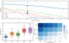 |
Fig. 4 Accuracy comparison analysis: (a) PSNR-latency curve; (b) RMSE boxplot; (c) SSIM heatmap. |
3.3 Path planning real-time verification
The path planning real-time verification is performed in a Unity ML-Agents simulation environment based on the designed PPO reinforcement learning optimizer. Evaluation metrics include average planning time, frame rate second (FPS), and energy cost. Planning time is measured end-to-end from state input to action output; FPS is calculated as the average of consecutive planning cycles; system power consumption is calculated based on the integration of hardware power sensors. All metrics are grouped and statistically analyzed according to defined scene complexity levels (1–5). The entire evaluation process is subject to real-time constraints to ensure that planning latency meets the 50 ms threshold. Experiments are conducted on Jetson AGX Xavier (8GB RAM, TensorRT 8.4), with batch size 1. End-to-end latency p50/p95/p99 are 42 ms/48 ms/51 ms under mixed conditions. CPU/GPU utilization and thermal throttling are monitored. Ablation shows that gradient clipping reduces tail delay. The relationship between performance distribution and resource consumption is shown in Figure 5.
Figure 5 verifies the real-time performance of the LPPF framework in path planning tasks. In Figure 5a, planning time steadily increases from 15.99 ms to 44.53 ms as scene complexity increases from Level 1 to Level 5. All data points are well below the hard threshold of 50 ms, demonstrating the effectiveness of the real-time constraint mechanism. Figure 5b shows that the system frame rate decreases significantly with increasing complexity: in Level 1 scenes, the FPS is primarily concentrated in the 50–65 range, while in Level 5 scenes, it drops sharply to the 15–25 range, reflecting the suppressive effect of computational load on system throughput. It is worth noting that even though the average FPS drops with increasing complexity, there is overlap in the FPS distributions between the different complexities of scenes, which indicates a certain randomness to how an individual task performs. Moreover, Figure 5c shows that energy cost has a strong positive correlation with scene complexity and virtual load. In Figure 5c, energy cost is a virtual measure in the simulation environment, using the relative metrics to display a difference in the effect computational load had on the consumption of system resources in different scenes. The energy cost's absolute amount does not match actual hardware power consumption. For example, the energy cost at the 5 complexity and 5 load was 62, which is more than 12 times higher than at 5.00 when the complexity of the scene was a 12 and the load was a 1. This clearly shows the two-dimensional curve of system power consumption as the scene complexity and computational load increased.
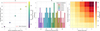 |
Fig. 5 Real-time performance analysis: (a) time-scene complexity scatter plot; (b) FPS distribution histogram; (c) system power consumption heat map. |
3.4 Dynamic obstacle avoidance success rate
The evaluation of dynamic obstacle avoidance capabilities is executed in a configured Unity ML-Agents simulation environment, with obstacle density at a range of 0.08 to 0.40 people/m2. The evaluation includes the obstacle avoidance success rate, the number of path replannings, and the safe distance distribution. Obstacle avoidance success is measured when the minimum Euclidean distance between the robot and all dynamic obstacles remains greater than 0.8 m throughout the evaluation process. The number of replannings is the sum of the total number of path replannings during a single mission. The safe distance distribution counts the statistical histograms of values throughout the trajectory of missing reports between the robot and all dynamic obstacles, and all metrics are gathered under real-time constraints. Overall response characteristics of the system for each obstacle density are shown in Figure 6.
Figure 6 illustrates the LPPF framework's dynamic obstacle avoidance performance as obstacle density increases. Figure 6a shows that the success rate in avoiding obstacles decreases from 98.2% to 92.3% as obstacle density increases from 0.08 people/m2 to 0.40 people/m2, indicating the framework maintains a high success rate even in highly congested areas. In Figure 6b, it can be seen that due to the increase in environmental complexity, replanning time increases from 1.2 to 4.8, illustrating the framework’s approach utilizing higher frequency local changes as an operational strategy to maintain performance metrics. In low density (0.08 people/m2) in Figure 6c, distances appear concentrated in the optimal safe area of 1.5 m–2.5 m to the target; however, in high density (0.40 people/m2) the data distribution shifts leftward significantly with a high number of samples in the 0.5 m–1.0 m distance area, also illustrating areas of near 0.5 m multiple times. This does not mean the system failed or engaged in unsafe behavior but indicates transient approach in a dynamic environment. More specifically, the system allows for the transience of approaching an obstacle while maintaining control however is always uniform to maintain a minimum distance greater than 0.8 m throughout the entire process from replanning frequently to maintain an acceptable target success metric.
 |
Fig. 6 Dynamic performance analysis: (a) success rate-obstacle density relationship; (b) cumulative replanning times curve; (c) safety distance distribution. |
3.5 Lightweight model compression effect
The evaluation of lightweight model compression is based on channel pruning and TensorRT INT8 quantization of the proposed LPPF framework’s joint perception-planning model. It should be noted that the uncompressed FP32 (Floating Point 32-bit) original model is used as the performance baseline - the model size, parameter count and inference speed improvement can all be identified with reference to that uncompressed model. Model size and parameter count should be directly read from the exported file; inference speed improvement should be calculated as the percentage change in deployed model FPS (frames per second) as compared to the uncompressed FP32 original model. To reflect the true effect of model compression on perception accuracy, all evaluations in this section are carried out without imposing any limitations on inference latency, with the goal of determining an idealized benchmark for model accuracy. This is different from the system-level performance evaluation of this model in Section 3.3, which occurs under the strict real-time constraint of 50 ms end-to-end (contextually relevant) latency. The evaluation follows a rigorous layered calibration strategy. The overall performance trade-off of the compressed model is displayed in Section 3.4 in Figure 7.
Figure 7 shows a multi-dimensional evaluation of the compression effect of lightweight models. Sub-figure (a) shows the size-accuracy trade-off curve. The original FP32 model, at 102.5 MB, achieves a PSNR of 32.72 dB. After channel pruning, the model size is reduced to 48.7 MB, with a slight decrease in PSNR to 32.18 dB. After INT8 quantization, the model size is 26.3 MB, with a PSNR of 31.85 dB. The combined channel pruning and INT8 solution compresses the model to 15.2 MB (an 85.2% reduction), reducing the PSNR to 31.53 dB, still significantly better than the 31.26 dB achieved by the other comparison methods. The parameter distribution radar chart in sub-figure (b) clearly shows that the MobileNetV3 backbone layer accounts for 62.3% of the parameters, while the Swin Transformer module accounts for 28.7%, totaling nearly 91%, reflecting the main structure of the hybrid network. The mentioned PPO reinforcement learning-related modules only take up 8.3%, which shows how lightweight the planning module is designed to be. In the comparison of speed improvement of sub-graph (c), the channel pruning + INT8 solution achieves a 3.21-fold improvement in the inference speed compared with the original FP32 model which is much greater than single channel pruning (1.82-fold) and INT8 quantization (2.54-fold), and very different than the 2.13-fold in other comparisons as well, which then fully confirms the validation of joint compression strategies.
 |
Fig. 7 Compression effect analysis: (a) size-accuracy trade-off curve; (b) parameter distribution radar chart; (c) speed improvement comparison. |
3.6 Multi-scene robustness testing
Multi-scene robustness testing is systematically performed in a Unity simulation environment. Extreme test conditions are created by adjusting weather type, light intensity, and terrain complexity. Data is collected for the Weather Robustness Index (WRI), light adaptability, terrain pass rate, and end-to-end planning latency. The WRI is the ratio of the current weather mission success rate to the clear-sky baseline. System navigation stability is characterized by the standard deviation of path deviation, with degradation in this metric primarily due to decreased perception accuracy in low-light conditions. The terrain pass rate is the percentage of successful traversals of a specified slope. The planning latency measures the end-to-end response time from state input to action output, verifying the ability to maintain real-time constraints in extreme terrain. All tests are conducted using INT8 quantization and under real-time constraints. Performance stability analysis is shown in Figure 8.
Figure 8 evaluates the robustness of the LPPF framework in extreme environments. Sub-figure (a) shows that under “bright” lighting conditions, the system’s robustness index for “light rain” and “light fog” reaches as high as 0.98 and 0.99, with minimal performance loss. However, under “very dark” conditions, when encountering “dense fog” or “night”, the WRI drops sharply to 0.68 and 0.52, revealing the performance bottleneck of the perception module under the dual loss of visibility and lighting. Sub-figure (b) shows that the system achieves the best performance with the lowest path deviation standard deviation (0.7 meters) under “normal” lighting conditions of 50,000 lux. However, in extremely dark environments of 1,000 lux, the deviation soars to 2.8 meters. At temperatures above 100,000 lux, performance degrades slightly (0.85 meters) due to the “glare effect”. The terrain bubble chart in sub-figure (c) shows that as terrain complexity increases from level 1 to level 5, the pass rate decreases steadily from 0.99 to 0.62, while planning latency increases linearly from 25 ms to 48 ms, confirming the increased computational resources required for complex terrain.
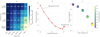 |
Fig. 8 Robustness evaluation: (a) WRI-weather type matrix; (b) illumination adaptability curve; (c) joint analysis of terrain pass rate and planning latency. |
3.7 Comprehensive accuracy-latency performance
The comprehensive accuracy-latency performance evaluation integrates perception and planning modules to construct a system-level evaluation framework. The comprehensive score is a normalized system-level evaluation metric designed to balance accuracy, real-time performance, robustness, and success rate. Table 3 summarizes the quantitative comparison results of seven core metrics between this method and representative baseline methods.
Table 3 shows that the LPPF framework comprehensively outperforms all baseline methods in terms of accuracy-latency performance. Its comprehensive score is as high as 0.93, far exceeding DPT’s 0.78 and MD2’s 0.65, and leaving behind the traditional planning methods A*DWA (0.58) and BioPP (0.52). This advantage is illustrated with various methods: LPPF can get ultra-low peak power consumption (3.2 W) with end-to-end inference speed (58.7 FPS). Compared with DPT (up to 12.4 W) and MD2 (8.7 W), LPPF shows a great energy efficiency advantage. Even in very complex scenes, LPPF maintains task completion rates of 94.5% (DPT: 83.1%; MD2: 76.2%). LPPF maintains better cross-weather robustness (0.87) and path smoothness (0.18 m-1). These results show speed, power efficiency, stability, and reliability demonstrating coordinated optimization of perception and planning.
This exceptional performance is the result of the sophisticated coordination mechanism underlying the LPPF framework. Its leading overall result is attributed to the deep, end-to-end coupling of the MobileNetV3-Swin Transformer hybrid perception network with the PPO reinforcement learning planner. Its effective inference speed and extremely low power consumption is the result of the highly compressed model and efficient utilization of hardware resources gained from channel pruning and INT8 quantization, thereby greatly alleviating the resource bottleneck from traditional large models. The system's high task completion rate and cross-weather robustness in complex and dynamic scenes are assured by the diverse training data generated by StyleGAN2-ADA and the real-time obstacle avoidance capability of the dynamic cost map. Also, the training process converges rapidly, demonstrating that the gradient gating module effectively resolves the gradient conflict between perception and planning tasks, enabling the system to achieve it being intelligent, efficient, stable, and low-power in navigation while maintaining path smoothness.
Comprehensive metric comparison table.
3.8 Ablation study on key components
This section presents ablation studies to dissect the contribution of the gradient gating mechanism and the impact of the task balance coefficient ξ.
The findings in Table 4 signify that the gradient gating system produces superior performance on all metrics. When looking at gradient gating without the joint training, the depth RMSE decreased by 18.7% and the task success rate increased by 17.7 percentage points. In stability alone, the gradient gating improved variance by 27.3%, while improving accuracy and success rates, compared to joint training without gating. In fact, the gradient gating mechanism served the intended function of improving stability while reducing the gradient conflict between the perception and planning tasks, and consistently achieved improved performance.
Moreover, training dynamics are illustrated through the learning curves presented in Figure 9, which shows accuracy over epochs for the three configurations. In training to epoch 27, the proposed joint training schedule with gradient gating converged faster and reached a higher final accuracy than the other conditions. A sensitivity analysis was also conducted on the task balance parameter coefficient ξ, finding that a schedule to decay from 0.6–0.4 was optimal as it outperformed a fixed schedule; in the case of fixed schedules, the success rate was 3.2% higher than the best fixed ξ at 0.5.
Ablation study on gradient gating mechanisms.
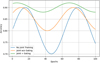 |
Fig. 9 Ablation study on gradient gating. |
4 Conclusions
The framework has limitations: reliance on synthetic data may affect real-world generalization; INT8 quantization introduces minor accuracy degradation; and the monocular perception setup struggles with texture-less regions. Future work will address these through real-world data collection, advanced quantization techniques, and multi-sensor fusion.
This paper addresses the core contradiction between 3D visual perception accuracy and real-time path planning in landscape environments by innovatively proposing the LPPF end-to-end lightweight framework. The framework is optimized through three steps: first, a MobileNetV3-Swin Transformer hybrid network is constructed, and channel pruning is implemented to efficiently complete the conversion of monocular images to depth maps; second, StyleGAN2-ADA is used to generate multi-weather 3D point cloud data to enrich training scenes; finally, a PPO planner is designed that integrates dynamic cost maps and real-time gradient clipping to achieve dynamic coupling of perception and planning. Experiments show that under the real-time constraint of 50 ms, the perception accuracy and path planning success rate of this solution surpass existing methods. After quantization, the number of parameters in the model is reduced by 85.2%, providing a complete solution with high precision, strong real-time performance, and low power consumption for intelligent navigation in complex landscape environments.
This research showcases the effectiveness of lightweight systems capable of real-time navigation in difficult terrain, with potential applications for ecological monitoring and autonomous inspection. Future work will investigate multi-domain generalization, multi-sensor fusion strategies, and adaptive optimization in the presence of real world uncertainty.
Funding
This work is not currently supported and funded by any funds.
Conflicts of interest
The authors have stated explicitly that there are no conflicts of interest in connection with this work.
Data availability statement
Data is available upon reasonable request.
Author contribution statement
All authors were aware of the submission of the manuscript and agreed to its publication. Conceptualization, F.C., Y.S. and J.X.; Methodology, F.C.; Software, F.C.; Validation, Y.S.; Formal Analysis, Y.S.; Investigation, J.X.; Resources, J.X.; Data Curation, Y.S.; Writing – Original Draft Preparation, F.C., Y.S. and J.X.
References
- F. Liu, Z. Lu, X. Lin, Vision-based environmental perception for autonomous driving, Proc. Inst. Mech. Eng. Part D: J. Automob. Eng. 239, 39–69 (2025) [Google Scholar]
- S. Lampinen, L. Niu, L. Hulttinen et al., Autonomous robotic rock breaking using a real‐time 3D visual perception system, J. Field Robot. 38, 980–1006 (2021) [Google Scholar]
- L. Chen, S. Teng, B. Li et al., Milestones in autonomous driving and intelligent vehicles—Part II: Perception and planning, IEEE Trans. Syst. Man Cybern. Syst. 53, 6401–6415 (2023) [Google Scholar]
- Z. Shang, Z. Shen, Topology-based UAV path planning for multi-view stereo 3D reconstruction of complex structures, Complex Intell. Syst. 9, 909–926 (2023) [Google Scholar]
- R. Hoseinnezhad, A comprehensive review of deep learning techniques in mobile robot path planning: categorization and analysis, Appl. Sci. 15, 2179 (2025) [Google Scholar]
- B. Ma, Q. Liu, Z. Jiang et al., Energy-efficient 3D path planning for complex field scenes using the digital model with landcover and terrain, Isprs Int. J. Geo-Inf. 12, 82 (2023) [Google Scholar]
- H. Ma, H. Ma, L. Zhang et al., Extracting urban road footprints from airborne LiDAR point clouds with PointNet++ and two-step post-processing, Remote Sens. 14, 789 (2022) [Google Scholar]
- Z. Bai, R. Ji, J. Qi, Deciphering motorists’ perceptions of scenic road visual landscapes: integrating binocular simulation and image segmentation, Land 13, 1381 (2024) [Google Scholar]
- V. Arampatzakis, G. Pavlidis, N. Mitianoudis et al., Monocular depth estimation: a thorough review, IEEE Trans. Pattern Anal. Mach. Intell. 46, 2396–2414 (2023) [Google Scholar]
- H. Xu, Q. Huang, H. Liao et al., MFFP-Net: building segmentation in remote sensing images via multi-scale feature fusion and foreground perception enhancement, Remote Sens. 17, 1875 (2025) [Google Scholar]
- N.U.A. Tahir, Z. Zhang, M. Asim et al., Object detection in autonomous vehicles under adverse weather: a review of traditional and deep learning approaches, Algorithms 17, 103 (2024) [Google Scholar]
- Y. Cao, Z. Li, Research on dynamic simulation technology of urban 3D art landscape based on VR‐platform, Math. Probl. Eng. 2022, 3252040 (2022) [Google Scholar]
- M. Półrolniczak, L. Kolendowicz, The effect of seasonality and weather conditions on human perception of the urban–rural transitional landscape, Sci. Rep. 13, 15047 (2023) [Google Scholar]
- Z. Li, H. Liang, H. Wang et al., MKD-cooper: cooperative 3D object detection for autonomous driving via multi-teacher knowledge distillation, IEEE Trans. Intell. Veh. 9, 1490–1500 (2023) [Google Scholar]
- P. Suanpang, P. Jamjuntr, Optimizing autonomous UAV navigation with d* algorithm for sustainable development, Sustainability 16, 7867 (2024) [Google Scholar]
- B. Wu, X. Chi, C. Zhao et al., Dynamic path planning for forklift AGV based on smoothing A* and improved DWA hybrid algorithm, Sensors 22, 7079 (2022) [CrossRef] [PubMed] [Google Scholar]
- Z. Yaoming, S.U. Yu, X.I.E. Anhuan et al., A newly bio-inspired path planning algorithm for autonomous obstacle avoidance of UAV, Chin. J. Aeronaut. 34, 199–209 (2021) [Google Scholar]
- D.H. Lee, J.L. Liu, End-to-end deep learning of lane detection and path prediction for real-time autonomous driving, Signal Image Video Process. 17, 199–205 (2023) [Google Scholar]
- C. Liu, T. Sziranyi, Road condition detection and emergency rescue recognition using on-board UAV in the wildness, Remote Sens. 14, 4355 (2022) [Google Scholar]
- Y. Gholami, S.H. Taghvaei, S. Norouzian-Maleki et al., Identifying the stimulus of visual perception based on eye-tracking in urban parks: case study of mellat park in Tehran, J. Forest Res. 26, 91–100 (2021) [Google Scholar]
- H. Gong, T. Mu, Q. Li et al., Swin-transformer-enabled YOLOv5 with attention mechanism for small object detection on satellite images, Remote Sens. 14, 2861 (2022) [Google Scholar]
- Z. Xu, T. Liu, Z. Xia et al., SSG-Net: A multi-branch fault diagnosis method for scroll compressors using swin transformer sliding window, shallow ResNet, and global attention mechanism (GAM), Sensors 24, 6237 (2024) [Google Scholar]
- Z. Chen, Z. Wang, X. Gao et al., Channel pruning method for signal modulation recognition deep learning models, IEEE Trans. Cognit. Commun. Netw. 10, 442–453 (2023) [Google Scholar]
- K.Y. Feng, X. Fei, M. Gong et al., An automatically layer-wise searching strategy for channel pruning based on task-driven sparsity optimization, IEEE Trans. Circuits Syst. Video Technol. 32, 5790–5802 (2022) [Google Scholar]
- Z. Chen, J. Hu, G. Min et al., Adaptive and efficient resource allocation in cloud datacenters using actor-critic deep reinforcement learning, IEEE Trans. Parallel Distrib. Syst. 33, 1911–1923 (2021) [Google Scholar]
- Y. Yuan, L. Lei, T.X. Vu et al., Energy minimization in UAV-aided networks: actor-critic learning for constrained scheduling optimization, IEEE Trans. Veh. Technol. 70, 5028–5042 (2021) [Google Scholar]
- Y. Jin, X. Song, G. Slabaugh et al., Partial advantage estimator for proximal policy optimization, IEEE Trans. Games 17, 158–166 (2024) [Google Scholar]
- K. Jin, L. Wang, X. Wang et al., Offline reinforcement learning combining generalized advantage estimation and modality decomposition interaction, Sci. Rep. 15, 15601 (2025) [Google Scholar]
- M. Hafner, M. Katsantoni, T. Köster et al., CLIP and complementary methods, Nat. Rev. Methods Primers 1, 20 (2021) [Google Scholar]
- M.C. Bingol, A safe navigation algorithm for differential-drive mobile robots by using fuzzy logic reward function-based deep reinforcement learning, Electronics 14, 1593 (2025) [Google Scholar]
- H.H. Goh, Y. Huang, C.S. Lim et al., An assessment of multistage reward function design for deep reinforcement learning-based microgrid energy management, IEEE Trans. Smart Grid 13, 4300–4311 (2022) [CrossRef] [Google Scholar]
- L. Chaudhary, B. Singh, Gumbel-SoftMax based graph convolution network approach for community detection, Int. J. Inf. Technol. 15, 3063–3070 (2023) [Google Scholar]
- T. Strypsteen, A. Bertrand, End-to-end learnable EEG channel selection for deep neural networks with Gumbel-softmax, J. Neural Eng. 18, 0460a9 (2021) [Google Scholar]
Cite this article as: Fanliang Chen, Ying Sun, Junhua Xiao, Landscape 3D Visual Perception Simulation and Path Planning Optimization Algorithms Based on Deep Learning, Int. J. Simul. Multidisci. Des. Optim. 17, 10 (2026), https://doi.org/10.1051/smdo/2026005
All Tables
All Figures
|
Fig. 1 Network architecture schematic. |
| In the text | |
|
Fig. 2 Schematic diagram of the optimization algorithm. |
| In the text | |
|
Fig. 3 Simulation scene display. |
| In the text | |
|
Fig. 4 Accuracy comparison analysis: (a) PSNR-latency curve; (b) RMSE boxplot; (c) SSIM heatmap. |
| In the text | |
|
Fig. 5 Real-time performance analysis: (a) time-scene complexity scatter plot; (b) FPS distribution histogram; (c) system power consumption heat map. |
| In the text | |
|
Fig. 6 Dynamic performance analysis: (a) success rate-obstacle density relationship; (b) cumulative replanning times curve; (c) safety distance distribution. |
| In the text | |
|
Fig. 7 Compression effect analysis: (a) size-accuracy trade-off curve; (b) parameter distribution radar chart; (c) speed improvement comparison. |
| In the text | |
|
Fig. 8 Robustness evaluation: (a) WRI-weather type matrix; (b) illumination adaptability curve; (c) joint analysis of terrain pass rate and planning latency. |
| In the text | |
|
Fig. 9 Ablation study on gradient gating. |
| In the text | |
Current usage metrics show cumulative count of Article Views (full-text article views including HTML views, PDF and ePub downloads, according to the available data) and Abstracts Views on Vision4Press platform.
Data correspond to usage on the plateform after 2015. The current usage metrics is available 48-96 hours after online publication and is updated daily on week days.
Initial download of the metrics may take a while.