")
")
| Issue |
Int. J. Simul. Multidisci. Des. Optim.
Volume 8, 2017
|
|
|---|---|---|
| Article Number | A11 | |
| Number of page(s) | 8 | |
| DOI | https://doi.org/10.1051/smdo/2017004 | |
| Published online | 2017年8月18日 | |
Research Article
Study of solutions to a class of certain parabolic systems with variable exponents
1
Research laboratory in Engineering (LRI), University Hassan II of Casablanca, National Higher School of Electricity and Mechanics (ENSEM), BP 8118, Oasis, Morocco
2
Département MIG, Ecole Hassania des Travaux Publics (EHTP), BP 8106, Oasis, Casablanca, Morocco
* e-mail: 该Email地址已收到反垃圾邮件插件保护。要显示它您需要在浏览器中启用JavaScript。
Received:
10
April
2017
Accepted:
22
June
2017
Abstract
In this paper, the authors study an initial and boundary value problem to a system of evolution p(x)-Laplacian systems coupled with general nonlinear terms:
ai(x)uit − div(|∇ui|pi(x)−2∇ui) = fi(x, u1, u2), (i = 1, 2).
The authors translate the parabolic equation into the elliptic equation by using the time discretization method, and then the existence and uniqueness solution are obtained. The blow-up results is shown, by using the energy method.
Key words: pi(x)-Laplacian systems / Existence / Uniqueness / Variable exponent / Blow-Up / Semi-discretization
© H. El Ouardi et al., published by EDP Sciences, 2017
 This is an Open Access article distributed under the terms of the Creative Commons Attribution License (http://creativecommons.org/licenses/by/4.0), which permits unrestricted use, distribution, and reproduction in any medium, provided the original work is properly cited.
1 Introduction
Let 
 (N ≥ 1) be a bounded Lipshitz domain and 0 < T < ∞. It will be assumed throughout this paper that p(x) is continuous function defined in
  with logarithmic module of continuity:
 (1)
(1)
We set Q
T
= Ω × (0, T) and Σ
T
= ∂Ω × (0, T). Our aim is to prove the existence and uniqueness of solutions u = (u
1, u
2) to the nonlinear (p
1(x), p
2(x))-Laplacian system: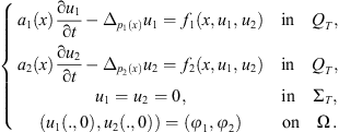 (2)where
  is a function, (i = 1, 2).
The operator 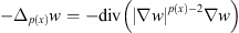 is called p(x)-Laplacian, which will be reduced to the p-Laplacian when p(x) = p a constant.
The (p
1(x), p
2(x))-Laplacian system (2) can be viewed as a generalization of (p, q)-Laplacian system (3)
(3)
For the case p i (x) = p i > 2, and a i (x) = 1, (i = 1, 2), system (2) models as non-Newtonian fluids [2, 21] and nonlinear filtration [2], etc. In the non-Newtonian fluids theory, (p 1, p 2) is a characteristic quantity of the fluids, there have been many results about the existence, uniqueness of the solutions. We refer the readers to the bibliography given in [7, 9, 10, 11, 28, 31] and the references therein.
In recent years, the research of nonlinear problems with variable exponent growth conditions has been an interesting topic. p(·)-growth problems can be regarded as a kind of nonstandard growth problems and these problems possess very complicated nonlinearities, for instance, the p(x)-Laplacian operator 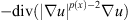 is inhomogeneous. And these problems have many important applications in nonlinear elastic, electrorheological fluids and image restoration. The reader can find in [14, 22] several models in mathematical physics where this class of problem appears.
The case of a single equation of the type (2) has been studied in [4–6, 20] and the authors established the existence and uniqueness results, in [20], the authors use the difference scheme to transform the parabolic problem to a sequence of elliptic problems and then obtain the existence of solutions with less constraint to p i (x).
The more interesting question concerning parabolic systems of (p 1(x), p 2(x))-Laplacian type is to understand the asymptotic behavior of solutions when time goes to infinity. The study of the asymptotic behavior of the system is giving us relevant information about the structure of the phenomenon described in the model.
Concerning the elliptic systems with variable exponents, the results about existence and non-existence are proved in [26, 27, 29, 30].
Note that system (2) has a more complicated nonlinearity than the classical (p,q)-Laplacian system since it is nonhomogenous.
Recently, [24] study the equation the p(x)-Laplacian equation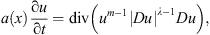 where λ > 0, m + λ − 2 > 0 and a(x) is a positive continuous function. They examine under which conditions on behavior of a(x) corresponding nonnegative solutions of the Cauchy problems possess the finite speed of propagations or interface blow-up phenomena.
In this paper, we consider the existence and uniqueness for the problem of the type (2) under some assumptions. The proof consists of two steps. First, we prove that the approximating problem admits a global solution; then we do some uniform estimates for these solutions. We mainly use skills of inequality estimation and the method of approximation solutions. By a standard limiting process, we obtain the existence to problem of the type (2).
The outline of this paper is the following: In Section 2, we introduce some basic Lebesgue and Sobolev spaces and state our main theorems. In Section 3, we give the existence and uniqueness of weak solutions. In Section 4, the blow-up results will be proved. The asymptotic behaviour of solution is established in Section 5.
2 Preliminaries
To consider problems with variable exponents, one needs the basic theory of spaces L p(x)(Ω) and W 1p(x)(Ω). For the convenience of readers, let us review them briefly here. The details and more properties of variable-exponent Lebesgue-Sobolev spaces can be found in [16, 17].
Let  When p
− > 1, one can introduce the variable-exponent Lebesgue space
When p
− > 1, one can introduce the variable-exponent Lebesgue space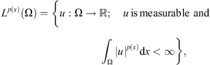 endowed with the Luxemburg norm.
The conjugate space is L
q(x)(Ω), with 

As in the case of a constant exponent, set endowed with the norm
Similarly we also denote by  the closure of
  in
in  and
and  is the dual of
  with respect to the inner product in
In Propositions 2.1–2.3, we describe some results about the Luxembourg norm.
-
The space
 is a separable, uniformly convex Banach space, and its conjugate space is
  where
where 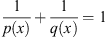
 For any
  and
and  we have the following Hölder-type inequality:

-
If
 for any
  the imbedding
 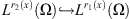 is continuous, the norm of the imbedding does not exceed
Proposition 2.2 [16]
If we denote then
then
-
|w|(r(x)) < 1(= 1; > 1) ⇔ ρ(w) < 1 (= 1; > 1);
-

-
|w|(r(x)) → 0 ⇔ ρ(w) → 0; |w|(r(x)) → ∞ ⇔ ρ(w) → ∞.
Proposition 2.3 [16]
For  there exists a constant
  such that:
This implies that  and
and  are equivalent norms of
System (2) does not admit classical solutions in general. So, we introduce weak solutions in the following sence.
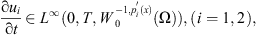
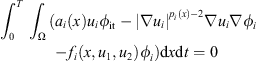
Definition 2.4 A function u = (u 1 , u 2) is said to be a weak solution of equation (2) , if the following conditions are satisfied:
-

 such that:
 -
For any

-

In the study of the global existence of solutions, we need the following hypotheses (H):
-
(H1)

-
(H2)

-
(H3)

3 Main results
Remark 3.1 In this paper, we shall denote by c i , C i differents constants, depending on p i (x), T, Ω, but not on n, which may vary from line to line. Sometimes we shall refer to a constant depending on specific parameters C i (T), etc.
Our main existence result is the following:
Theorem 3.2 Let (H1)–(H3) hold. Then system (2) admits a unique solution u = (u 1 ,u 2 ) ∈ (C((0, T); L 2(Ω)))2 . Moreover, the mapping (φ 1, φ 2) → (u 1(t), u 2(t)) is continuous in L 2(Ω) × L 2(Ω).
Proof of the main results.
3.1 Existence
We will semi-discrete (2) in time and solve the corresponding elliptic problem. Based on the semi-discrete problem, we construct the corresponding approximate solutions. The key procedure is to establish necessary a priori estimates for finding the limit of the approximate solutions via a compactness argument.
We first consider the discrete scheme (4)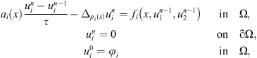 (4)where Nτ = T and T is a fixed positive real, and 1 ≤ n ≤ N.
Lemma 3.3
For any fixed n, if
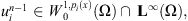 Problem (4) admits a weak solution
Proof. On the space  we consider the functional
 where
where  is a known function. Using Young’s inequality and Proposition 2.1, there exist constants C
1, C
2 > 0, such that:
is a known function. Using Young’s inequality and Proposition 2.1, there exist constants C
1, C
2 > 0, such that: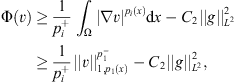 hence Φ(v) → ∞, as
  Since the norm is lower semi-continuous and
  is continuous functional, Φ(v) is weakly lower semi-continuous on
  and satisfy the coercive condition. From [14] we conclude that there exists
  such that:
 and v* is the weak solutions of the Euler equation corresponding to Φ(v),
Choosing  we obtain a weak solution
  of (4).
 (5)
(5)
Since  , we may prove by induction that (4) has a solution
  in
in  We put
  and for any integer k > 0, we may take
  as a test function in (5) to get
By using the Hölder inequality and  , we have
We deduce 
Letting k → ∞, we get  Consider
  , we get easily that
  , i.e.
  and if we choose
  such that
  , we obtain
This completes the proof of lemma 3.3.
Now, we define the approximate solutions as 
 set by: for all n ∈ {1, …, N}.
![Mathematical equation: $$ \forall t\in \left[(n-1)\tau,{n\tau }\right]\enspace \left\{\begin{array}{l}{u}_{{i\tau }}(t)={u}_i^n,\enspace \\ \\ {\mathop{u}\limits^\tilde}_{{i\tau }}(t)=\frac{\left(t-\left(n-1\right)\tau \right)}{\tau }\left({u}_i^n-{u}_i^{n-1}\right)+{u}_i^{n-1},\end{array}\right. $$](/articles/smdo/full_html/2017/01/smdo170002/smdo170002-eq87.gif) are well defined and satisfied in addition
are well defined and satisfied in addition (6)
(6)
We first establish some energy estimates of  .
.
We need several lemmas to complete the proof of Theorem 3.2.
Lemma 3.4
There exists a positive constant C(T, u
0) such that, for all n = 1, …, N
 (7)
(7)
 (8)
(8)
 (9)and
 (10)
(10)
Proof. (a) By lemma 3.3, for any n ∈ N,  is bounded; whence (7)
(b) Multiplying (4) by  , summing from n = 1 to N and integrating over Ω, we obtain
 (11)
(11)
By using the Young inequality, for  small, there exists
  such that
 (12)
(12)
With the aid of the identity 2α(α − β) = α
2 − β
2 + (α − β)2, we get
With the above estimates, we get (8).
(c) Multiplying the equation (4) by  and summing from n = 1 to N, we get
By using the Young inequality, we get (13)
(13)
From the convexity of the expression  we get the following inequality:
 (14)
(14)
which imply with (12) and (13) that
By lemma 3.4, there exists M
i
> 0 independent of  such that:
 (15)
(15)
Therefore, taking  and up to subsequence, we get that there exists
  such that
  , and as
  ,
, (16)
(16)
 (17)
(17)
From (14), it follows that u
i
= v
i
. From (15), we get that (18)
(18)
By Aubin-Simon’s compactness results [22], we have (19)
(19)
Now, multiplying (4) by  and using (14) and (15), we get by straightforward calculations:
 where
where  as
as  .
.
Thus, we get that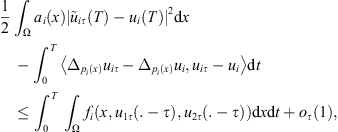 (20)and from (16) we have thus,
 and consequently by the same as that in [24]
Therefore, u i satisfies (3).
3.2 Uniqueness
Let (H1)–(H3) be satisfied. Then system (2) has a unique solution u = (u 1, u 2) in Q T.
Proof. Let u = (u
1, u
2) and v = (v
1, v
2) be solutions of (2), we have:
Since f
i
(x,.,.) is locally Lipschitz uniformly in Ω, the difference w
i
= u
i
− v
i
satisfies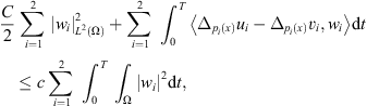 we observe that w → −Δ
p(x)
w is monotone from
we observe that w → −Δ
p(x)
w is monotone from  to
to 
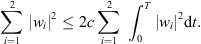 (21)
(21)
We finally deduce from Gronwall’s lemma,
Thus, we deduce that u i = v i .
Thus the solution is unique. The continuity of the the mapping  can be obtained similarly.
Remark 3.5
From Theorem 3.2, the solution of system (2) generates a semigroup
 in L
2(Ω) × L
2(Ω).
in L
2(Ω) × L
2(Ω).
Remark 3.6
If we assume that f
i
(x, s
1, s
2) = g
i
(x, s
1, s
2) − h
i
(x, s
i
) where
 is Carathéodory mapping and that there exist positive constants L
j
, c
j
, m
j
, C
j
such that:
is Carathéodory mapping and that there exist positive constants L
j
, c
j
, m
j
, C
j
such that:
-
 for any x ∈ Ω and
-
 for any x ∈ Ω and
  where
where  with
with  and
and 
 with
with  and
and 
By the same argument as that in [12, 32], One can show in the same way that the semigroup  associated with system (2) admits an absorbing set in
  there is a bounded set
  such that, for any bounded set B in L
2(Ω) × L
2(Ω), there exists a T
0 > 0 such that
such that, for any bounded set B in L
2(Ω) × L
2(Ω), there exists a T
0 > 0 such that  for any t ≥ T
0. Where T
0 depends only on B.
for any t ≥ T
0. Where T
0 depends only on B.
4 Blow-up of solutions
In this section, we shall investigate the blow-up properties of solutions to system (2) using energy methods. To this end, we consider the following hypotheses on the data.
(H4)  such that:
(H5)  and H is such that:
Throughout this section, we define for t ≥ 0
Theorem 4.1
Let (H1)–(H5) be satisfied, then the solutions of system (2) blow up in finite time, namely, there exists a T* < ∞ such that
 as t → T*.
Proof. We define 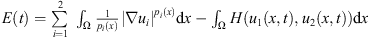 .
.
Multiplying the first equation of (2) by  , the second by
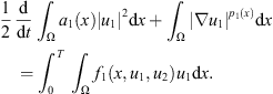
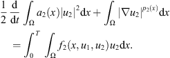
  , integrating by parts, we have
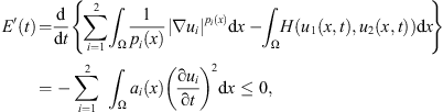 (22)which implies that E(t) ≤ E(0).
Next define 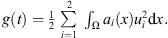
Multiplying the first equation of (2) by u
1, the second by u
2, integrating by parts, we have (23)
(23)
By using Hölder’s inequality, we have (24)where
By the formula  we have by combining (23), (24)
 where
where 
A direct integration of the above inequality over (0, t) then yields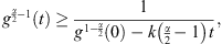 which implies that g(t) bows up at a finite time
 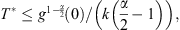 and so does u
i
.
and so does u
i
.
5 Asymptotic behaviour
This section is devoted to the asymptotic behaviour of solutions. In order to prove the asymptotic behaviour, we assume
(H6) 
Theorem 5.1
The weak solution u = (u
1(t), u
2(t)) obtained in Theorem 3.2, satifies:  where C
i
> 0 (i = 1, 2, 3),
where C
i
> 0 (i = 1, 2, 3), 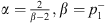 or
or  or
or  .
.
Proof. Let u i be solution of (2).
Multiplying the first equation in (2) by u
1 and integrating over Q
T
, (25)
(25)
Multiplying the second equation in (2) by u
2 and integrating over Q
T
, (26)
(26)
Summing up (25) and (26), we have from hypothesis (H5) that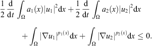 (27)
(27)
By u
i
 using Poincaré’s inequality, we obtain
 (28)
(28)
If  and
and  by Proposition 2.2,
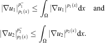 (29)
(29)
According to the assumption that p
1(x) ≤ p
2(x), Then 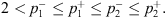
Hence, we get from (28) that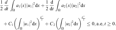 (30)
(30)
By the formula  we have
![Mathematical equation: $$ {\left(\frac{1}{2}{\int }_{\mathrm{\Omega }} \left[{\left|{u}_1\right|}^2\mathrm{d}x+{\left|{u}_2\right|}^2\right]\mathrm{d}x\right)}^{\frac{{p}^{-}}{2}}\le C{\left({\int }_{\mathrm{\Omega }} {\left|\nabla {u}_1\right|}^{{p}_1(x)}\mathrm{d}x\right)}^{\frac{{p}^{-}}{2}}+{\left({\int }_{\mathrm{\Omega }} {\left|\nabla {u}_2\right|}^{{p}_2(x)}\mathrm{d}x\right)}^{\frac{{p}^{-}}{2}}, $$](/articles/smdo/full_html/2017/01/smdo170002/smdo170002-eq182.gif) (31)this implies that
(31)this implies that![Mathematical equation: $$ \frac{1}{2}\frac{\mathrm{d}}{\mathrm{d}t}{\int }_{\mathrm{\Omega }} {\left|{u}_1\right|}^2\mathrm{d}x+\frac{1}{2}\frac{\mathrm{d}}{\mathrm{d}t}{\int }_{\mathrm{\Omega }} {\left|{u}_2\right|}^2\mathrm{d}x+{C}_3{\left({\int }_{\mathrm{\Omega }} \left[{\left|{u}_1\right|}^2\mathrm{d}x+{\left|{u}_2\right|}^2\right]\mathrm{d}x\right)}^{\frac{{p}^{-}}{2}}\le 0,a.e,t\ge 0, $$](/articles/smdo/full_html/2017/01/smdo170002/smdo170002-eq183.gif) (32)where C
3 = min(C
1, C
2).
(32)where C
3 = min(C
1, C
2).
Denote![Mathematical equation: $$ h(t)={\int }_{\mathrm{\Omega }} \left[{\left|{u}_1\right|}^2\mathrm{d}x+{\left|{u}_2\right|}^2\right]\mathrm{d}x. $$](/articles/smdo/full_html/2017/01/smdo170002/smdo170002-eq184.gif)
Then, we obtain from (32) and (H2) that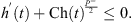 (33)
(33)
If  and
and  by Proposition 2.2,
Then we get from (28) that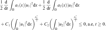 (34)
(34)
That is![Mathematical equation: $$ \frac{1}{2}\frac{\mathrm{d}}{\mathrm{d}t}{\int }_{\mathrm{\Omega }} {a}_1(x){\left|{u}_1\right|}^2\mathrm{d}x+\frac{1}{2}\frac{\mathrm{d}}{\mathrm{d}t}{\int }_{\mathrm{\Omega }} {a}_2(x){\left|{u}_2\right|}^2\mathrm{d}x+{C}_3{\left({\int }_{\mathrm{\Omega }} \left[{\left|{u}_1\right|}^2\mathrm{d}x+{\left|{u}_2\right|}^2\right]\mathrm{d}x\right)}^{\frac{{p}_2^{+}}{2}}\le 0,a.e,t\ge 0. $$](/articles/smdo/full_html/2017/01/smdo170002/smdo170002-eq190.gif) (35)
(35)
Again we have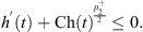
Similarly, if  and
and  or
or  and
and  we can also obtain the similar results
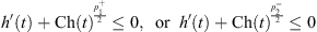
Hence![Mathematical equation: $$ {\int }_{\mathrm{\Omega }} \left[{\left|{u}_1\right|}^2\mathrm{d}x+{\left|{u}_2\right|}^2\right]\mathrm{d}x\le \frac{{C}_1}{{\left({C}_2t+{C}_3\right)}^{\alpha }},\enspace \alpha =\frac{2}{\beta -2},\beta ={p}_1^{-}\enspace \mathrm{or}\enspace {p}_2^{+}\enspace \mathrm{or}\enspace {p}_2^{-},{C}_i>0,\enspace i=\mathrm{1,2},3. $$](/articles/smdo/full_html/2017/01/smdo170002/smdo170002-eq197.gif)
The proof is complete.
References
- Astrita G, Marrucci G. 1974. Principles of non-Newtonian fluid mechanics. McGraw-Hill: New York. [Google Scholar]
- Acerbi E, Mingine G. 2002. Regularity results for stationary electrorheological fluids. Arch. Ration. Mech. Anal., 164, 213–259. [CrossRef] [MathSciNet] [Google Scholar]
- Acerbi E, Mingione G, Seregin GA. 2004. Regularity results for parabolic systems related to a class of non Newtonian fluids. Ann. Ins. H. Poincaré Anal. Non Linéaire, 21, 25–60. [Google Scholar]
- Antontsev SN, Shmarev SI. 2009. Anisotropic parabolic equations with variable nonlinearity. Publ. Mat., 53(2), 355–399. [CrossRef] [MathSciNet] [Google Scholar]
- Antontsev SN, Shmarev SI. 2005. A model porous medium equation with variable exponent of nonlinearity: existence, uniqueness and localization properties of solutions. Nonlinear Anal., 60, 515–545. [CrossRef] [MathSciNet] [Google Scholar]
- Antontsev SN, Shmarev SI. 2009. Localization of solutions of anisotropic parabolic equations. Nonlinear Anal., 71, 725–737. [CrossRef] [Google Scholar]
- El Ouardi H, de Thelin F. 1989. Supersolutions and stabilization of the solutions of a nonlinear parabolic system. Publicacions Mathematiques, 33, 369–381. [CrossRef] [MathSciNet] [Google Scholar]
- El Ouardi H, El Hachimi A. 2002. Existence and regularity of a global attractor for doubly nonlinear parabolic equations. Electron. J. Diff. Eqns., 2002(45), 1–15. [Google Scholar]
- El Ouardi H, El Hachimi A. 2001. Existence and attractors of solutions for nonlinear parabolic systems. Electron. J. Qual. Theory Differ. Equ., 5, 1–16. [CrossRef] [EDP Sciences] [MathSciNet] [Google Scholar]
- El Ouardi H, El Hachimi A. 2006. Attractors for a class of doubly nonlinear parabolic systems. Electron. J. Qual. Theory Differ. Equ., 1, 1–15. [Google Scholar]
- El Ouardi H. 2011. Global attractor for quasilinear parabolic systems involving weighted p-Laplacian operators. J. Pure App. Mat. Advances App., 5(2), 79–97. [MathSciNet] [Google Scholar]
- El Ouardi H. 2013. Long-time behavior for a nonlinear parabolic systems with variable exponent of nonlinearity. Int. J. Adv. Math. Math. Sci., 2(1), 27–36. [Google Scholar]
- Esteban JR, Vazquez JL. 1982. On the equation of turbulent filtration in one-dimensional porous media. Nonlinear Anal., 10, 1303–1325. [CrossRef] [Google Scholar]
- Kristaly A, Radulescu V, Varga C. 2010. Variational principles in mathematical physics, geometry, and economics. Qualitative analysis of nonlinear equations and unilateral problems in Encyclopedia of mathematics and its applications, vol. 136. Cambridge University Press: Cambridge. [Google Scholar]
- Chang KC. 1986. Critical point theory and its applications. Shanghai Scientific and Technology Press: Shanghai. [Google Scholar]
- Fan X. 2007. Global C1,α regularity for variable exponent elliptic equations in divergence form. J. Diff. Equ., 235, 397–417. [CrossRef] [Google Scholar]
- Fan X, Zhao D. 2001. On the space Lp(x)(Ω) and Wm,p(x) (Ω). J. Math. Anal. Appl., 263, 749–760. [CrossRef] [Google Scholar]
- Fan X, Zhang QH. 2003. Existence of solutions for p(x)-Laplacian Dirichlet problem. Nonlinear Anal., 52, 1843–1852. [CrossRef] [MathSciNet] [Google Scholar]
- Lions JL. 1969. Quelques méthodes de résolution des problèmes aux limites non linéaires. Dunod: Paris. [Google Scholar]
- Lian S, Gao W, Yuan H, Cao C. 2012. Existence of solutions to an initial problem of evolutional p(x)-Laplace equations. Ann. I. H. Poincaré – AN, 29(3), 377–399, DOI: 10.1016/j.anihpc.2012.01.001. [CrossRef] [MathSciNet] [Google Scholar]
- Martinson LK, Pavlov KB. 1971. Unsteady shear flows of a conducting fluid with a rheological power law. Magnitnaya Gidrodinamika, 2, 50–58. [Google Scholar]
- Ruzicka M. 2000. Electrorheological fluids: Modeling and mathematical theory. Lecture Notes in Mathematics. vol. 1748. Berlin: Springer-Verlag. [CrossRef] [Google Scholar]
- Simon J. 1987. Compact sets in Lp(0, T; B). Ann. Mat. Pura Appl., 146, 65–96. [Google Scholar]
- Tedeev AF. 2007. The interface blow-up phenomenon and local estimates for doubly degenerate parabolic equation. Appl. Anal., 86(6), 755. [CrossRef] [MathSciNet] [Google Scholar]
- Zhao JN. 1993. Existence and nonexistence of solutions for ut = div(|∇u|p − 2∇u) + f(∇u, u, x, t). J. Math. Anal. Appl., 172(1), 130–146. [CrossRef] [MathSciNet] [Google Scholar]
- Fu Y, Zhang X. 2009. Multiple solutions for a class of p(x)-Laplacian systems. J. Inequal. Appl. Art., 2009(191649), 1–12. [Google Scholar]
- El Hamidi A. 2004. Existence results to elliptic systems with non standard growth condition. J. Math. Anal. Appl., 300, 30–42. [CrossRef] [MathSciNet] [Google Scholar]
- Marion M. 1987. Attractors for reaction-diffusion equation: existence and estimate of their dimension. Appl. Anal., 25, 101–147. [CrossRef] [MathSciNet] [Google Scholar]
- Ogras S, Mashiyev A, Avci M, Yucedag Z. 2008. Existence of solution for a class of elliptic systems in RN involving the (p(x), q(x))-Laplacian. J. Inequal. Appl., 612938, 16. [MathSciNet] [Google Scholar]
- Xu X, An Y. 2008. Existence and multiplicity of solutions for elliptic systems with nonstandard growth conditions in RN. Nonlinear Anal., 68, 956–968. [CrossRef] [MathSciNet] [Google Scholar]
- Wei Y, Gao W. 2007. Existence and uniqueness of local solutions to a class of quasilinear degenerate parabolic systems. Appl. Math. Comput., 190, 1250–1257. [CrossRef] [MathSciNet] [Google Scholar]
- Niu W. 2012. Long-time behavior for a nonlinear parabolic problem with variable exponents. J. Math. Anal. Appl., 393, 56–65. [CrossRef] [MathSciNet] [Google Scholar]
Cite this article as: El Ouardi H & Ghabbar Y: Study of solutions to a class of certain parabolic systems with variable exponents. Int. J. Simul. Multisci. Des. Optim., 2017, 8, A11.
Current usage metrics show cumulative count of Article Views (full-text article views including HTML views, PDF and ePub downloads, according to the available data) and Abstracts Views on Vision4Press platform.
Data correspond to usage on the plateform after 2015. The current usage metrics is available 48-96 hours after online publication and is updated daily on week days.
Initial download of the metrics may take a while.