")
")
| Issue |
Int. J. Simul. Multidisci. Des. Optim.
Volume 15, 2024
|
|
|---|---|---|
| Article Number | 17 | |
| Number of page(s) | 12 | |
| DOI | https://doi.org/10.1051/smdo/2024015 | |
| Published online | 15 October 2024 | |
Research Article
Structural damage recognition based on wavelet transform and improved most valuable player algorithm
School of Intelligent Manufacturing, Anhui Vocational And Technical College, Hefei 230011, China
* e-mail: This email address is being protected from spambots. You need JavaScript enabled to view it.
Received:
10
April
2024
Accepted:
6
August
2024
Abstract
The probability of damage to infrastructure increases with age. Timely health monitoring of infrastructure is essential since it is linked to the safety of people's lives and property. The study employed the wavelet transform approach to discretize the wavelet transform of the observed vibration patterns of the damaged structure in order to identify and localize the structural damage in infrastructure. The study also employed natural excitation techniques to obtain the structural multi-order modal parameters. To quantify the degree of structural damage, the study designed an objective function for damage quantification and improved the most valuable player algorithm. The study avoided the most valuable player algorithm from falling into local optimality by introducing the elite inverse strategy and simplex strategy. The wavelet transform and the improved most valuable player algorithm were able to successfully identify and localize the structural damages and quantify the degree of the damages, thereby providing technical support for the daily monitoring of the infrastructure.
Key words: Wavelet transform / most valuable player algorithm / structural damage identification / degree quantification / localization
© Y. Li, Published by EDP Sciences, 2024
 This is an Open Access article distributed under the terms of the Creative Commons Attribution License (https://creativecommons.org/licenses/by/4.0), which permits unrestricted use, distribution, and reproduction in any medium, provided the original work is properly cited.
1 Introduction
As the economy develops and society advances, so does the construction of infrastructure. Whether it is a new or long-established infrastructure, its own safety is very important. Therefore, advanced techniques are needed for Structural Damage (SD) identification and Degree Quantification (DQ) of infrastructure [1]. For identification of SD, Modal Parameters (MPs) need to be identified and inferences about the condition of the structure are made from these MPs. MPs contain various kinds, such as Vibration Mode (VM), frequency, etc. The random subspace approach, time series method, Hilbert-Yellow transform method, and other methods are frequently used to identify MPs [2,3]. With the development of technology, Wavelet Function (WF) is gradually applied to the identification of MPs, and the specific methods include amplitude extraction method, singular value decomposition method, wavelet packet method, curvature modal method, and vibration modal method, etc. [4]. The singular value decomposition method has good ability to remove early noise and has high recognition accuracy. For the calculation of SD cases, the common methods are model correction method, neural network method, strain modal, and principal component analysis method [5]. Moreover, some researchers have developed intelligent composite materials that can monitor the health status and performance of structures, and have yielded promising outcomes [6]. These studies do, however, have some drawbacks, including the vibration modal method's insensitivity to singularities, the algorithm's propensity to settle into the local optimum, and the lack of adequate attention to external conditions. Therefore, the study employs Wavelet Transform (WT) to Discrete Wavelet Transform (DWT) the vibration patterns identified by the damage structure. The study also designed the Objective Function (OF) for damage quantification and improved the Most Valuable Player Algorithm (MVPA) by introducing Elite Reverse Strategy (ERS) and Simplex Strategy (SimS). The innovations of the study are mainly in two aspects. The first is the introduction of ERS and SimS, and the second is the integrated use of WT and improved MVPA. The study aims to provide technical support for the daily damage monitoring of infrastructure, to ensure the safety of infrastructure, and to safeguard the lives and properties of the people. The experimental results revealed that the wavelet coefficient corresponding to measurement point 6 was the largest with a value of 1.68 in the identification of damage location for transverse first-order vibration patterns. It is feasible to localize the damage location by wavelet transform with high accuracy. The minimum values of the Average Fitness Values (AFVs) of the improved most valuable player algorithm were 10−15 and 10−16.7 on different multi-peak functions (MPFs). The study is broken up into four sections altogether. The first section is a review of previous research on SD detection and DQ. The second part is the specific design of WT and improved MVPA. The third part is the validation of the effectiveness of WT and improved MVPA. The fourth part is the conclusion, shortcomings, and outlook of the study.
2 Related works
With the development of society and economy, the construction of infrastructure is also developing simultaneously. The safety of infrastructure is related to the personal and property safety of each of us, so more and more experts have launched research on the identification and DQ of SD. To identify and localize crack damage in subway bogies, Zhang Y et al. designed a guided wave based IoT method to perform simple and effective damage detection through inexpensive piezoelectric ceramic sensor network. The method was performed without removing paint contamination for damage detection. The method's effectiveness in identifying the extent and position of damage to the bogie plate frame was demonstrated by the testing findings, which also showed that the recognition was more sensitive for small area damage [7]. Zhu J et al. created a detection technique that uses just two sensors to identify bridge degradation. The damage index was defined by the approach, which was based on the transfer entropy of bridge information. According to the experimental results, the approach had a good detection impact when it came to identifying bridge damage in both single and multiple damage scenarios [8]. Ai Y et al. used the acoustic emission technique and the support vector machine to identify and categorize the feature parameters in order to track the on-rail tensile damage of gearbox housing materials. According to the testing data, the degradation model was able to correctly identify the damage and predict the life, and the approach developed for this study had a classification accuracy of more than 90% [9]. To address the shortcomings of the Jaya technique, such as the absence of excitation measurements for SD identification and the challenges associated with parameter selection in the conventional Tikhonov regularization approach, Zhang G. et al. developed an iterative approach. The study designed an improved L-curve method and the method was based on the B-spline interpolation function. The outcomes revealed that the strategy designed in this study performed well in terms of the location and degree of SD and the improved Jaya algorithm performed better compared to the baseline algorithm [10].
Lei J et al. designed a detection method combining vibration statistical indicators and support vector machines in order to identify the SD, defining a variety of structural scenarios, and the scenarios also included the absence of SD. To obtain the acceleration response, the study placed sensors at each level of the structure. The outcomes indicated that the method designed by the study was able to provide a better identification of damage features and was robust in terms of noise immunity [11]. To better identify the SD, Li XY et al., fused the existing identification results to obtain the advantages of various damage indices and assessment methods. Experimental results revealed that a large number of sensors were required to achieve high spatial resolution of localized damage when mathematical models of the structure were not used [12]. To determine the SD of the components and connectors, Ramezani M. et al. created a modified genetic algorithm for the location and degree of damage. The method was based on a finite number of modes and healthy elements were identified and removed. The performance validation of the method was mainly realized by two numerical examples. The experimental results showed that the approach was noise-free and can identify damage with a limited number of modalities [13]. Wang X et al. combined the Hilbert-Yellow transform and convolutional neural network for the recognition of SD. The damage signals of the baseline model were analyzed in this study using the Hilbert-Yellow transform, and the analysis's output was fed into the convolutional neural network model. According to the experimental results, the damage identification approach provided in this study is more superior, and the optimized convolutional neural network model's performance is also somewhat enhanced [14].
In summary, the current studies on SD recognition are relatively rich and use a variety of methods. However, these studies also have certain shortcomings, such as insufficient consideration of environmental factors, and the selection of sensor locations can be further explored. Therefore, the study employs WT to identify the location of the SD and uses a natural excitation technique to obtain the structural multi-order MPs. In addition, the study also designed the OF for damage quantification and improved the MVPA by introducing ERS and SimS.
3 Location identification and degree quantification method design for structural damage
The study shows how to calculate the intrinsic frequency of the structure and creates the WT method to make DWT of the vibration pattern detected by the damaged structure in order to determine the location of SD. For the quantification of the degree of SD, the study constructs an OF for damage quantification and designs a modified MVPA to optimize the calculation.
3.1 Design of structural damage position recognition based on wavelet transform
For location identification and DQ of SD, the study first uses the WT method to identify the damaged structure, and later on the modified MVPA is used to quantify the SD. To identify the SD of infrastructure building works, the study adopts the WT method to make DWT of the identified VMs of the damaged structure. The study utilizes sensors to obtain the acceleration response information at different locations. In order to obtain the multi-order MPs of the structure, the study adopts the natural excitation technique, and the calculation of the intrinsic frequency of the structure is illustrated. As a widely used technique for signal analysis, the Fourier Transform (FT) can effectively represent the features of signals in the frequency domain and transfer data between the temporal and frequency domains. Unfortunately, this approach is unable to view data in both the frequency and temporal domains at the same time [15,16]. To solve this problem, the short-time FT and WT came into being. Short-time FT is able to observe the time-frequency domain simultaneously, but it also has the problem that the window width cannot be changed flexibly [17]. WT not only can realize the time-frequency conversion of the signal, but also because the wavelet in WT has its own “width,” so the window width will be adjusted according to the specific wavelet width [18]. WT can make up for the shortage of short-time FT, and has the flexibility and scale conversion, so the research adopts the method of WT. In WT, a wavelet called “mother wavelet” is selected first, and a “wavelet cluster” can be obtained from the “mother wavelet”. The composed wavelet cluster is shown in equation (1) [19].
 (1)
(1)
In equation (1), a and b represent arbitrary real numbers, ϕ(t) denotes the mother wavelet, and t is the time. Equation (2) displays the wavelet basis's time window center [20].
 (2)
(2)
In equation (2), ϕa,b(t) stands for wavelet clusters, and d is the basic symbol of calculus, i.e., differentiation. Equation (3) shows the width of the temporal window [21].
 (3)
(3)
In equation (3), t0 represents the center of the time window. Equation (4) displays the frequency window center [22].
 (4)
(4)
In equation (4), ω represents the frequency, ψ (ω) represents the FT, and ψa,b (ω) denotes the FT of the wavelet basis after telescoping and translating. Since the wavelet basis function has the zoom property, it is able to provide a better identification of the singularity. Equation (5) displays the WT for signal f(t).
 (5)
(5)
In equation (5), p represents the expansion factor, q represents the translation factor, ϕ' (t) is the selected wavelet basis function, and WTf represents the wavelet coefficients of the signal after WT. There are two main types of WT methods, continuous WT and DWT. However, continuous WT has high redundancy and huge computation. DWT reduces the computational volume by discretizing the translation and expansion factors, and the discretized WF is shown in equation (6) [23].
 (6)
(6)
In equation (6), n and m represent the scaling factor and translation factor of the discrete wavelet, respectively. Equation (7) displays signal f(t)'s DWT.
 (7)
(7)
DWT can be used in signal denoising, signal recognition and diagnosis, so the study adopts DWT in WT for SD recognition. However, the computation of DWT is still relatively large, so the study uses the multi-resolution analysis method and Mallat algorithm to improve the computation speed of DWT. Multi resolution analysis requires spatial sequences that satisfy five properties, as shown in Figure 1.
In Figure 1, the five properties that multi-resolution analysis needs to satisfy are consistent monotonicity, asymptotic completeness, scaling regularity, translation invariance, and existence of orthogonal basis. The main concept of the multiresolution analysis is to remove the complimentary features from the signal such that just the signal's backbone remains. The use of multiresolution analysis method does not require WF, which can improve the speed of computation. The Mallat algorithm treats the input signal as an initial approximation component, and through the high- and low-pass filter, it can realize the multi-scale decomposition of the signal, which can improve the speed of computation. There are seven common WFs, as shown in Figure 2.
From Figure 2, the WF is mainly categorized into Haar wavelet, Morlet wavelet, Daubechies wavelet, Mexican Hat wavelet, Meyer wavelet, Symlets wavelet, and biorthogonal wavelet. In SD identification, obtaining the MPs of the structure from the response data is a very crucial step. The identification of MPs mainly contains the identification of frequency and VM. The steps of identification of MPs are shown in Figure 3.
In Figure 3, the identification of MPs is divided into four main steps, which are frequency identification, VM identification, data processing and selection of WF. In the identification of frequency, the study adopts the natural excitation technique with complex Morlet WT for the mutual correlation function. The complex Morlet WT can be employed for continuous WT. It incorporates amplitude and phase parameters that are straightforward to correlate with the characteristics of the signal. Therefore, the complex Morlet WT is often used for parameter identification of structural modes. Equation (8) presents the results of the structure's z A th order frequency computation.
 (8)
(8)
In equation (8), fs represents the sampling frequency of the response signal and fc represents the center frequency of the complex Morlet wavelet. αz is the scale of WT corresponding to the intrinsic frequency of the structure. In the identification of VMs, the ratio of wavelet coefficients corresponding to the αz scale can be used to obtain the VM information of the order. The values of the VMs at different translational scales are not necessarily the same, so they need to be normalized.
 |
Fig. 1 Five properties that multi-resolution analysis needs to satisfy. |
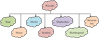 |
Fig. 2 Types of wavelet functions. |
 |
Fig. 3 Steps for identifying modal parameters. |
3.2 Degree quantification design for structural damage based on improved MVPA
In the previous section, the study designed a WT-based SD location identification method. In this section, the study will design the improved MVPA for SDDQ. Before designing the improved MVPA, the study needs to define the OF for damage quantification. When damage occurs in a structure, the vibration characteristics of the structure itself will change. The most commonly utilized damage characterization indexes are structural intrinsic frequency, modal flexibility, modal curvature, and modal VM. Among these, structural intrinsic frequency and modal VM are the most frequently employed indexes [24]. Structural intrinsic frequency has the advantages of being less affected by noise, easy to measure, and relatively less dependent on measurement information. However, the sensitivity of structural intrinsic frequency on small damage is low. Modal vibration patterns are sensitive to local variations in the structure and can compensate for the lack of structural intrinsic frequency. The data from these metrics enable backward reasoning about the extent of SD. Therefore, the study will use the structural intrinsic frequency and modal vibration pattern to construct the OF. The OF is shown in equation (9).
 (9)
(9)
In equation (9), Θω represents the function based on the intrinsic frequency of the structure, and δω is the weight in the OF. Θθ represents the function based on the VM, and δθ is the weight in the OF. g denotes the damage state vector of all units of the structure. The expression of the function based on the intrinsic frequency of the structure is shown in equation (10).
 (10)
(10)
In equation (10), Rω represents the frequency order required to form the OF, and  and
and  represent the zth order intrinsic frequency before and after the change, respectively. The expression of the function based on the vibration pattern is shown in equation (11).
 (11)
(11)
In equation (11), Rθ represents the number of orders of vibration patterns required to form the OF.  represents the correlation between the analyzed vibration pattern of the zth order structure and the measured vibration pattern of the zth order structure, and its value ranges from [0,1]. The calculation of
  is shown in equation (12).
 (12)
(12)
In equation (12),  represents the analyzed vibration pattern of the zth order.
  represents the zth order measured vibration pattern, and ∥∥ is the Euclidean parameter. The modified OF is shown in equation (13).
 (13)
(13)
In equation (13), coupling represents the intrinsic frequency as a function of the coupling to the VM, Ry represents the desired modal order, and F(g) is the penalty function. The calculation of coupling is shown in equation (14).
 (14)
(14)
In equation (14), RootMSEz represents the root mean square error. For the design of optimization algorithm in damage quantification stage, MVPA is selected for the study. The flow of the standard MVPA is shown in Figure 4.
Initializing the algorithm parameters, such as the number of athletes, teams, and iteration steps maximum, is the first stage of the typical MVPA in Figure 4. Assigning teams and initializing the athletes' skills is the second phase. The athletes on the team have their Fitness Values (FVs) calculated in the third phase, and the individual competition between the athletes is conducted in the fourth. The fifth step is to perform team competition between teams, and the sixth step is to run the greedy mechanism and elite strategy. Duplicate athletes with the same skills are removed in the seventh step, and the termination condition is checked in the eighth. The process ends and the ideal athlete is produced if it is fulfilled. If it is not satisfied, the operation of adding 1 to the number of iteration steps is performed, after which it returns to the third step. The representation of each player in the MVPA algorithm is shown in equation (15) [25].
 (15)
(15)
In equation (15), k represents the kth player, problemsize denotes the dimension of the problem, and S is the skill. The expression of a team composed of players is shown in equation (16).
 (16)
(16)
In equation (16), playersize represents the number of players in the league. The MVPA has few parameters, a high success rate, and a quick convergence speed. Nonetheless, it will enter a local optimum in complex problems, which will lead to poor convergence accuracy [26,27]. Therefore, the study will use ERS and SimS to improve MVPA in order to increase its overall optimization performance. The specific improvement measures are to consider the solution in the opposite direction through ERS and to avoid the premature convergence of MVPA through the characteristics of SimS geometric transformation to achieve the effect of finding the global optimal solution. The effect of ERS in improving the performance of swarm intelligence algorithms is more significant [28]. The schematic of the simplex is shown in Figure 5.
In Figure 5, xg represents the global optimal solution and xb represents the global suboptimal solution. xs is the solution to be replaced. xr is the reflection point. xc is the intermediate point between xg and xb. xe is the expansion point. xt is the compression point, and xw is the Contraction Point (CP). The specific process of the simplex is shown in Figure 6.
In Figure 6, the first step of the simplex is to evaluate all the solutions in the population and select xg and xb. The second step is to compute the FVs of xg, xb and xs. Assessing the intermediate points is the third phase. Getting the reflection point xr and figuring out the matching FVs is the fourth step. The fifth step is to determine whether the FV of xr is smaller than the FV of xg. If it is smaller, then the calculation of the expansion point will be carried out. Otherwise, the process will resume with the fourth step. The sixth step is to determine whether the FV of xr is smaller than the FV of xs. If it is smaller, then replace xs with the compression point, otherwise replace xs with the reflection point. The seventh step is to determine whether the FV of xg < reflection point xr < is satisfied. If so, calculate the FV of the CP. Otherwise, go back to the fourth step. The eighth step is to determine whether the FV of the CP is less than the FV of the xs. If so, replace the xs with the CP, otherwise replace the xs with the reflection point, and finally end the process.
 |
Fig. 4 The process of the standard MVPA. |
 |
Fig. 5 The diagram of a simplex. |
 |
Fig. 6 The specific process of simplex. |
4 Location identification of structural damage and analysis of degree quantification results
This section presents an analysis of the SD location identification results. Specifically, the study employs the transverse and longitudinal wavelet coefficients for several VMs to identify the precise location of the SD. The study performs a function test to examine the adaptive convergence curve and variance of the improved MVPA in order to confirm the enhanced MVPA's efficacy on the DQ of the SD.
4.1 Structural damage location identification results based on wavelet transform
The study chooses a high-speed train station in a city for simulation in order to assess the efficacy of WT on SD location detection. Accelerometer sensors are employed to collect reaction data for the structural model, and Ansys software is used in the study to simulate this HSR station. There are 15 sensors on the transverse line and 18 sensors on the longitudinal line in the platform-level plane of the station. After obtaining the acceleration data from different measurement points, in order to process the data, the study will calculate the cross-correlation between the acceleration of the two measurement points by the natural excitation method and treat the cross-correlation function as the signal to be analyzed for continuous WT. In order to identify the SDs, the study sets up six working conditions, each of which corresponds to a different load and damage location, etc. The study also uses the Windows 11 operating system as the operating system for the experiments. The operating system used for the experiment is Windows 11, and the processor is an Intel Core i5-13600K processor with a maximum memory of 192 GB. The specific conditions of different working conditions are shown in Table 1.
In Table 1, the load types for all the conditions are white noise, except for Case B. The load type for Case B is non-white noise. The load location for all cases is the centerline of the roof except for Case C. The load location for Case C is the entire roof. The load location for Case C is the entire roof. No damage occurred in conditions A, B, and C. Damage occurred in conditions D, E, and F. The loads in conditions D, E, and F are the entire roof. The damage locations for cases D, E, and F are all set on flat surfaces, and the damage levels are set to 30%, 15%, and 60%, respectively. The acceleration response signals at nodes 12069 and 12557 of the anomalous input signals are selected for the third-order discrete WT. The schematic diagram of the deformation of simply supported beams under stress and the explanation of different working conditions are shown in Figure 7.
In Figure 7a, when a simply supported beam is subjected to external forces, it will bend and be damaged on its own. In Figure 7b, different operating conditions correspond to different positions. The results of identifying the transverse damage locations under Case 4 are shown in Figure 8.
In Figure 8a, in the transverse first-order Vibration Damage Location Identification (VDLI), the wavelet coefficient corresponding to measurement point 6 is the largest, with a value of 1.68. With a value of 0.02, the wavelet coefficients that correspond to measurement points 1 and 15 are the smallest. In Figure 8b, in the transverse second-order VDLI, the wavelet coefficient corresponding to measurement point 4 is the largest, with a value of 0.28. In Figure 8c, in the transverse fourth-order vibration, the wavelet coefficient of measurement point 2 is the largest, with a value of 0.37 × 10⁻⁴. In Figure 8d, the wavelet coefficient of measurement point 9 is the largest, with a value of 0.25, in the identification of the damage location of the transverse sixth-order vibration pattern. The measurement points with the largest wavelet coefficient and the pre-set damage location correspond to each other, which demonstrates that the use of the WT to locate the damage location is feasible and has a high accuracy. This shows that it is feasible to use WT to localize the damage location with high accuracy. Figure 9 displays the results of the identification of the Longitudinal Damage Location (LDL) in working condition 4.
In Figure 9a, in the longitudinal first-order VDLI, the wavelet coefficient corresponding to measurement point 15 is the largest, with the value of 467.68. In the longitudinal second-order VDLI, the wavelet coefficient corresponding to measurement point 12 is the largest, with a value of 16.25. From Figure 9(b), in the fourth-order damage location identification, the wavelet coefficient corresponding to measurement point 16 is the largest, with a value of 8.57. In the sixth-order damage location identification, the wavelet coefficient corresponding to measurement point 15 is the largest, with a value of 17.36. In the LDL identification, the measurement points with the largest values and the preset damage locations also correspond to each other. In the sixth-order damage location identification, measurement point 15 has the largest wavelet coefficient, with a value of 17.36. In the LDL identification, the measurement points with the largest wavelet coefficients correspond to the predefined damage locations, which shows that the WT has a high accuracy in damage location localization.
Specific situations of different working conditions.
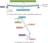 |
Fig. 7 Schematic diagram of stress and deformation of simply supported beams and explanation of different working conditions. |
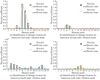 |
Fig. 8 Identification results of lateral damage location under condition 4. |
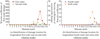 |
Fig. 9 Identification results of LDL under working condition 4. |
4.2 Degree quantification results for structural damage based on improved MVPA
To verify the effectiveness of the improved MVPA on the DQ of SD, the study conducted function tests, which are Single-Peak Function (SPF) and MPF. The variable dimension of both the single-peak and MPFs is 30 and the global minimum is 0. The comparison algorithms selected for the study are Gravitational Search Algorithm (GSA), Grey Wolf Optimizer (GWO), and Flower Pollination Algorithm (FPA), and each of the algorithm is run independently. The experimental environment is the same as in the previous section, and the programming tool is Matlab R2018(b). The convergence curves of the fitness of the different algorithms under the SPF are shown in Figure 10.
Through Figure 10a, it can be noticed that the Minimum Value (Min-V) of the AFV of the GSA algorithm is 10−8, the Min-V of the AFV of the FPA is 10−18, the Min-V of the AFV of the GWO algorithm is 10−28, the Min-V of the AFV of the MVPA is 10–18, and the Min-V of the AFV of the improved MVPA is 10−325. As the iterations increase, the AFV of the five algorithms also decreases, among which the AFV of the improved MVPA decreases at the fastest rate. From Figure 10b, the minimum AFVs of GSA, GWO, and FPAs are 10−2, 10−17 and 1 respectively. Moreover, the minimum AFVs of MVPA before and after the improvement are 10−9 and 10−170 respectively. The maximum AFV of the MVPA is 102, and that of the other four algorithms is all 1. This shows that the improved MVPA performs better. Comparison of adaptation convergence curves of different algorithms under MPF is shown in Figure 11.
From Figure 11a, the Maximum Value (Max-V) of the AFV of the GSA algorithm is 1 and the Min-V is 10−1.5. The Max-V of the AFV of the FPA and the GWO algorithm are 0.82 and 10.25, respectively, and the Min-Vs are 0.72 and 10−13, respectively. The Max-V of the AFV before and after the improvement of the MVPA are 10.25 and 1.27, respectively, and the Min-Vs are are 10−9.8 and 10−15, respectively. The improved MVPA plateaus after almost 180 iterations, while the MVPA and GWO algorithm plateau after almost 400 and 350 iterations, respectively. In Figure 11b, the Max-Vs of the AFVs of the GSA algorithm, the FPA, and the GWO algorithm are 102.9, 1, and 102.9, respectively, and the Min-Vs are 101.5, 10−1.5, and 10−2.4, respectively. The Max-Vs of the AFVs of the MVPA before and after the improvement are 102.9 and 102, respectively, and the Min-Vs are 10−16.7, respectively. The ANOVA of the different algorithms on the single-peak and MPFs is shown in Figure 12.
In Figure 12a, the Max-V of the variance of the GSA algorithm is 3.12 and the Min-V is 0. The Max-V of the variance of the FPA is 4.98 and the Min-V is 3.04. The Max-V of the variance of the GWO algorithm, the MVPA, and the improved MVPA are 0 and the Min-V is 0. In Figure 12b, the Max-V of the variance of the GSA algorithm is 50 and the Min-V is 15 for the MPF. In Figure 12b, on the MPF, the Max-V of variance of the GSA algorithm is 50, and the Min-V is 15. The Max-V of variance of FPA is 70, and the Min-V is 3. The Max-V of variance of the GWO algorithm is 20, and the Min-V is 0. The Max-V of variance of MVPA before and after the improvement and Min-V of variance of improved MVPA are both 0, and the fluctuation of variance of the improved MVPA is less, and it is more stable. This indicates that the enhanced MVPA's overall performance is more consistent.
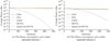 |
Fig. 10 Convergence curves for fitness of several methods under unimodal functions. |
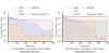 |
Fig. 11 Comparison of fitness convergence curves of different algorithms under multimodal functions. |
 |
Fig. 12 Analysis of variance of different algorithms on unimodal and multimodal functions. |
5 Conclusion
To identify and localize the damage in the structure and to DQ the SD, the study made discrete WT of the vibration patterns identified from the damaged structure and improved the MVPA. The experimental results revealed that the Max-Vs of the wavelet coefficients were 1.68, 0.28, 0.37 × 10⁻⁴ and 0.25 in the horizontal first-order, second-order, fourth-order and sixth-order vibration pattern damage location identification. The Max-Vs of the wavelet coefficients were 467.68, 16.25, 8.57 and 17.36 in the longitudinal first-order, second-order, fourth-order and sixth-order vibration pattern damage location identification. It can be concluded from this that that it was feasible to utilize WT to locate the damage location with high accuracy. The Min-Vs of the AFVs of the improved MVPA were 10−325 and 10−170 for different single peak functions, respectively. The Min-Vs of the AFVs of the improved MVPA were 10−15 and 10−16.7 under different MPFs. On the SPF, the Max-Vs of the variance of the improved MVPA were all 0, and the Min-Vs were all 0. On the MPF, the fluctuation of the variance of the improved MVPA was smaller and more stable. This reveals that the overall performance of the improved MVPA is more stable. The study considers less mathematical theoretical proofs on the convergence and computational complexity of MVPA. It is recommended that future studies conduct more in-depth research on MVPA and broaden the application areas of MVPA. Furthermore, the impact of the external environment has not received as much attention in this work. Future research can concentrate on how the external environment affects the intrinsic frequency of the structure.
Funding
This research received no specific grant from any funding agency in the public, commercial, or not-for-profit sectors.
Conflicts of interest
The author declares that there is no conflicts of interest.
Data availability statement
The data used to support the findings of the research are available from the corresponding author upon reasonable request.
Author contribution statement
Yan Li: Study design, data collection, statistical analysis, visualization, writing, and revision of the manuscript.
References
- Y. Zhang, Q. Hao, G. Cai, J. Lv, C. Yang, Crack damage identification and localisation on metro train bogie frame in IoT using guided waves, IET Intell. Transport Syst. 14, 1403–1409 (2020) [CrossRef] [Google Scholar]
- J. Zhu, W. Cai, Using two sensors for damage detection of bridge based on transfer entropy of vehicle-bridge information, J. Build. Technol. 3, 29–42 (2022) [CrossRef] [Google Scholar]
- G. Zhang, C. Wan, L. Xie, S. Xue, Structural damage identification with output-only measurements using modified Jaya algorithm and Tikhonov regularization method, Smart Struct. Syst. 31, 229–245 2023 [Google Scholar]
- V.H.L. Tirumani, M. Tenneti, K.C. Srikavya, S.K. Kotamraju, Image resolution and contrast enhancement with optimal brightness compensation using wavelet transforms and particle swarm optimization. IET Image Process. 15, 2833–2840 (2021) [CrossRef] [Google Scholar]
- J. Lei, Y. Cui, W. Shi, Structural damage identification method based on vibration statistical indicators and support vector machine, Adv. Struct. Eng. 25, 1310–1322 (2022) [CrossRef] [Google Scholar]
- H. Herranen, J. Majak, P. Tsukrejev, K. Karjust, O. Mrtens, Design and Manufacturing of composite laminates with structural health monitoring capabilities, Proc. CIRP 72, 647–652 (2018) [CrossRef] [Google Scholar]
- Y. Zhang, Q. Hao, G. Cai, J. Lv, C. Yang, Crack damage identification and localisation on metro train bogie frame in IoT using guided waves, IET Intell. Transport Syst. 14, 1403–1409 (2020) [CrossRef] [Google Scholar]
- J. Zhu, W. Cai, Using two sensors for damage detection of bridge based on transfer entropy of vehicle-bridge information, J. Build. Technol. 3, 29–42 (2022) [CrossRef] [Google Scholar]
- Y. Ai, Y. Zhang, H. Cui, W. Zhang, Characterization, identification and life prediction of acoustic emission signals of tensile damage for HSR gearbox housing material, Railway Sci. 2, 225–242 (2023) [CrossRef] [Google Scholar]
- G. Zhang, C. Wan, L. Xie, S. Xue, Structural damage identification with output-only measurements using modified Jaya algorithm and Tikhonov regularization method, Smart Struct. Syst. 31, 229–245 (2023) [Google Scholar]
- J. Lei, Y. Cui, W. Shi, Structural damage identification method based on vibration statistical indicators and support vector machine, Adv. Struct. Eng. 25, 1310–1322 (2022) [CrossRef] [Google Scholar]
- X.Y. Li, S.J. Lin, S.S. Law, Y.Z. Lin, J.F. Lin, Fusion of structural damage identification results from different test scenarios and evaluation indices in structural health monitoring, Struct. Health Monitor. 20, 2540–2565 (2021) [CrossRef] [Google Scholar]
- M. Ramezani, O. Bahar, Structural damage identification for elements and connections using an improved genetic algorithm, Smart Struct. Syst. 28, 643–660 (2021) [Google Scholar]
- X. Wang, X. Zhang, M.M. Shahzad, A novel structural damage identification scheme based on deep learning framework. Structures 29, 1537–1549 (2021) [CrossRef] [Google Scholar]
- S. Veerasingam, M. Ranjani, R. Venkatachalapathy, A. Bagaev, V. Mukhanov, D. Litvinyuk, P. Vethamony, Contributions of Fourier transform infrared spectroscopy in microplastic pollution research: a review, Crit. Rev. Environ. Sci. Technol. 51, 2681–2743 (2021) [CrossRef] [Google Scholar]
- K. Skrai, J. Petrovi, P. Pale, Classification of low- and high-entropy file fragments using randomness measures and discrete Fourier transform coefficients, Vietnam J. Comput. Sci. 10, 433–462 (2023) [CrossRef] [Google Scholar]
- R.M. Zhang, X. Xu, D.G. Truhlar, Observing intramolecular vibrational energy redistribution via the short-time Fourier transform, J. Phys. Chem. A 126, 3006–3014 (2022) [CrossRef] [Google Scholar]
- M. Grobbelaar, S. Phadikar, E. Ghaderpour, A.F. Struck, N. Sinha, R. Ghosh, M.Z.I. Ahmed, A survey on denoising techniques of electroencephalogram signals using wavelet transform, Signals 3, 577–586 (2022) [CrossRef] [Google Scholar]
- L.P.A. Arts, E.L.V.D. Broek, The fast continuous wavelet transformation (fCWT) for real-time, high-quality, noise-resistant time-frequency analysis, Nat. Comput. Sci. 2, 47–58 (2022) [CrossRef] [Google Scholar]
- V. Gupta, Wavelet transform and vector machines as emerging tools for computational medicine, J. Ambient Intell. Human. Comput. 14, 4595–4605 (2023) [CrossRef] [Google Scholar]
- C. Ghosh, A. Verma, P. Verma, Real time fault detection in railway tracks using fast Fourier transformation and discrete wavelet transformation, Int. J. Inf. Technol. 14, 31–40 (2022) [Google Scholar]
- J. Luo, S. Liu, Z. Cai, C. Xiong, G. Tu, A multi-task learning model for non-intrusive load monitoring based on discrete wavelet transform, J. Supercomput. 79, 9021–9046 (2023) [CrossRef] [Google Scholar]
- G.B. Gebremeskel, A critical analysis of the multi-focus image fusion using discrete wavelet transform and computer vision, Soft Comput. 26, 5209–5225 (2022) [CrossRef] [Google Scholar]
- M.H. Daneshvar, M. Saffarian, H. Jahangir, H. Sarmadi, Damage identification of structural systems by modal strain energy and an optimization-based iterative regularization method, Eng. Comput, 39, 2067–2087 (2023) [CrossRef] [Google Scholar]
- D. Bassir, H. Lodge, H. Chang, J. Majak, G. Chen, Application of artificial intelligence and machine learning for BIM, Int. J. Simul. Multidiscip. Des. Optim. 14, 5 (2023) [CrossRef] [EDP Sciences] [Google Scholar]
- H. Mokayed, T.Z. Quan, L. Alkhaled, V. Sivakumar, Real-time human detection and counting system using deep learning computer vision techniques, Artif. Intell. Appl. 1, 221–229 (2023) [Google Scholar]
- N. Vijaya Anand, J. Hema Latha, G. Devadasu, C. Kumar, Generation of optimal switching angle for nine level cascaded H bridge MLI using most valuable player algorithm, Turk. J. Comput. Math. Educ. 12, 1919–1927 (2021) [Google Scholar]
- B.S. Yildiz, N. Pholdee, S. Bureerat, A.R. Yildiz, S.M. Sait, Enhanced grasshopper optimization algorithm using elite opposition-based learning for solving real-world engineering problems, Eng. Comput. 38, 4207–4219 (2022) [CrossRef] [Google Scholar]
Cite this article as: Yan Li, Structural damage recognition based on wavelet transform and improved most valuable player algorithm, Int. J. Simul. Multidisci. Des. Optim. 15, 17 (2024)
All Tables
All Figures
|
Fig. 1 Five properties that multi-resolution analysis needs to satisfy. |
| In the text | |
|
Fig. 2 Types of wavelet functions. |
| In the text | |
|
Fig. 3 Steps for identifying modal parameters. |
| In the text | |
|
Fig. 4 The process of the standard MVPA. |
| In the text | |
|
Fig. 5 The diagram of a simplex. |
| In the text | |
|
Fig. 6 The specific process of simplex. |
| In the text | |
|
Fig. 7 Schematic diagram of stress and deformation of simply supported beams and explanation of different working conditions. |
| In the text | |
|
Fig. 8 Identification results of lateral damage location under condition 4. |
| In the text | |
|
Fig. 9 Identification results of LDL under working condition 4. |
| In the text | |
|
Fig. 10 Convergence curves for fitness of several methods under unimodal functions. |
| In the text | |
|
Fig. 11 Comparison of fitness convergence curves of different algorithms under multimodal functions. |
| In the text | |
|
Fig. 12 Analysis of variance of different algorithms on unimodal and multimodal functions. |
| In the text | |
Current usage metrics show cumulative count of Article Views (full-text article views including HTML views, PDF and ePub downloads, according to the available data) and Abstracts Views on Vision4Press platform.
Data correspond to usage on the plateform after 2015. The current usage metrics is available 48-96 hours after online publication and is updated daily on week days.
Initial download of the metrics may take a while.