| Issue |
Int. J. Simul. Multidisci. Des. Optim.
Volume 14, 2023
|
|
|---|---|---|
| Article Number | 18 | |
| Number of page(s) | 12 | |
| DOI | https://doi.org/10.1051/smdo/2023020 | |
| Published online | 14 December 2023 | |
Research Article
Simulation analysis of structural nonlinear seismic response
School of Civil Engineering and Architecture, Kaifeng University, Kaifeng, 475004, China
* e-mail: This email address is being protected from spambots. You need JavaScript enabled to view it.
Received:
20
September
2023
Accepted:
12
November
2023
Abstract
Faced with the difficulty of analyzing structural nonlinear seismic response, this study focuses on the reinforced concrete frame structure and designs a frame that meets the specifications. Artificial synthetic seismic records and natural seismic records were selected, and the acceleration response of the first story of the structure was used as the output sample for the study. On the basis of a nonlinear autoregressive moving average model with external inputs, a neural network model was constructed and nonlinear seismic response simulation analysis was conducted. These results confirm that the research method has good predictive performance and can effectively predict structural nonlinear seismic response. Under the action of artificial earthquake records, there is a small difference between them and the acceleration time history curve and acceleration response peak obtained from time history analysis. Under the action of artificial seismic record ACC12, when the time is 25 s, the calculation results of time history analysis and research methods are 1.715 m/s2 and 1.403 m/s2, respectively, with the former being 0.312 m/s2 smaller than the latter. In natural earthquake records, with a characteristic period of 0.30 s, under the action of natural earthquake record USA00668, the relative energy of time history analysis is 4.997 m2/s when the time is 30 s, which is 0.938 m2/s higher than the research method. The research method can accurately analyze the nonlinear seismic response of the results.
Key words: Nonlinearity / seismic response / neural network / simulation analysis
© F. Qin, published by EDP Sciences, 2023
 This is an Open Access article distributed under the terms of the Creative Commons Attribution License (https://creativecommons.org/licenses/by/4.0), which permits unrestricted use, distribution, and reproduction in any medium, provided the original work is properly cited.
1 Introduction
In recent years, bridges, super high-rise buildings, and large-span spatial structures have developed rapidly in China. The emergence of such structures often goes beyond the current regulations in China, and is also the case in international and domestic theoretical research. Currently, there have been a large number of numerical simulations and model experiments. However, whether it can accurately grasp its true stress state and stress environment, whether it can be ignored in engineering design, whether it can ignore certain stress states and failure forms, and whether it can bring potential safety risks are important issues that urgently need to be solved [1–3]. During service, structural damage and even sudden accidents can occur due to fatigue, corrosion, material aging, and seismic effects. Once they occur, not only will they cause huge economic losses, but they will also have serious political and social consequences. Therefore, it is necessary to conduct damage identification, health diagnosis, safety evaluation, and disaster warning for existing large structures and equipment, and develop predictive maintenance and emergency maintenance systems. These are effective ways to eliminate safety hazards and avoid disasters and accidents. Analyzing the non-linear seismic response (NSR) of structures from these accidents has always been a focus of attention in the engineering community [4–6]. In in-depth research, estimating the seismic response of structures through relevant computational simulation tools is a good research method. Therefore, in order to understand the situation of structural nonlinear seismic response (SNSR), from the perspective of computational simulation tools, considering the advantages of neural networks (NN) in dealing with nonlinear problems in structural engineering, this study applies it to research in the hope of contributing to SNSR. The study consists of four parts. Firstly, there is a literature review that introduces the research status of domestic and foreign scholars on SNSR analysis and the application of NN in the seismic field. Then, by preparing the sample set, a relevant NN was constructed based on the nonlinear system model, and SNSR analysis was performed using this NN. The third part analyzes the application of the constructed NN. Finally, the research methods and results were summarized, and the research shortcomings and directions were pointed out.
In structures such as bridges and super high-rise buildings, they are affected by earthquakes, corrosion, and other factors, resulting in a certain degree of damage to these structures, thereby affecting the safety of people's lives and property. Therefore, it is necessary to analyze the NSR of this structure. Cattari et al. constructed a corresponding nonlinear model based on the relevant plane steel structure to analyze the relationship between seismic collision and its nonlinear response when facing torsion coupled buildings under the condition of flexible foundation. They utilized relevant ground motion records, analyzed adjacent structures, and compared different nonlinear dynamic response results to explore the related effects of earthquake collision and torsional eccentricity. From the relevant results, the situation where the outer frame is located is the most dangerous after an earthquake collision [7]. Cattari et al. analyzed the research progress in NSR of masonry structures. Although numerical models can evaluate the seismic resistance of buildings, this alone is not enough in the behavior analysis of masonry structures. Modelers also need to have a thorough understanding of the software used and possess a wide range of modeling software. In addition, important issues related to in plane and out of plane response modeling in masonry modeling were explored, and numerical examples were used to illustrate them. The use of comprehensive methods is beneficial to the development of research to a certain extent [8]. Alam et al. analyzed the flexible side failure behavior of the corresponding reinforced concrete structure when facing the problem of seismic failure of planar asymmetric structures. And they monitored its specific situation through fiber Bragg grating sensors and conducted finite element analysis. From the relevant results obtained, in the flexible side of the studied structure, special designs were made for seismic structures, which have a certain resistance to extreme earthquake events [9]. Huang et al. conducted relevant nonlinear research to analyze soil structure interaction. They reflected the flexible foundation on a half space nonlinear foundation through relevant flexibility functions. Under the action of discrete-time recursive filtering method, the functions were transformed into time domain, and non iterative algorithms were used to ensure displacement continuity and force balance, which were implemented through a finite element framework. These results confirm that the proposed method can quickly evaluate the seismic structural response and has good application results [10].
Zhang et al. conducted relevant research on the problem of automatic modeling of seismic story velocity using convolutional NN (CNN). The input of the model was set as velocity spectrum, and the corresponding model was constructed based on regularization. From the application effect of the model, it is more suitable for complex structures with low signal-to-noise ratio [11]. To quickly estimate the source parameters in micro seismic earthquakes, Nooshiri et al. applied CNN to compact two CNNs and aggregate features through fully connected NN to obtain the complete moment tensor and spatial position of the source. After application analysis, it has been confirmed that the solution obtained by the proposed method is consistent with the inversion solution under the standard method [12]. Wang et al. used deep CNN to denoise seismic data, which has residual learning features and requires preprocessing of the data between different methods. These results confirm that the noise suppression effect is good [13]. Li et al. faced the problem of structural damage detection and proposed corresponding detection methods based on CNN. Under the action of the transfer function of response data, the influence of relevant seismic excitation was eliminated. In the model input, the data was sourced from the structural response transfer rate data. After simulation analysis, it has been confirmed that the proposed model has good detection performance and can accurately detect structural damage [14].
In summary, in SNSR analysis, flexibility based methods and other methods cannot reflect the real-time changes in the degree of nonlinearity of the structure, while NN method does not have this problem. It only needs to train the excitation and structural response, and simulate and predict the seismic response of the structure based on the training results. Therefore, when studying the NSR simulation problem of structures, NN is applied to it.
2 SNSR analysis based on NN
To understand the NSR situation of the structure, the research focuses on reinforced concrete frame structures and conducts corresponding simulation analysis using NN. Prior to this, NN training samples were prepared, and the results of elastic-plastic time history analysis were used as the output signal of the training samples. A suitable NN model was selected and NN simulation program was developed. On this basis, NSR simulation was conducted.
2.1 Preparation of sample set
Analyzing the NSR of a structure is an important part of structural seismic engineering [15,16]. The research focuses on reinforced concrete frame structures and conducts NSR simulation analysis using the IDARC program for calculating damage indices. In this program, the model used is a dual parameter failure model. The selection of structure was carried out, and a three span, six story reinforced concrete frame structure was selected for research. Figure 1 shows its plane layout and facade layout.
In Figure 1, a 6 m*6 m column grid is used. For the bottom story, its height is set to 4.5 m, and each story in the remaining stories is 3.9 m. The live load on the floor is set to 2.0 kN/m2, and the live load on the accessible roof is set to 2.0 kN/m2. Considering the symmetry of the structural layout, a mid-span plane element is selected for NSR analysis. In the framework, fully cast-in-place beams, slabs, and columns were selected, with a concrete strength grade of C30 and a corresponding slab thickness of 120 mm. The cross-sectional dimensions were adjusted to meet the requirements, resulting in the final dimensions in Figure 2.
In Figure 2, except for the bottom story, the cross-sectional dimensions of all other stories are the same. In the natural vibration period of the structure, the calculation results using PKPM software show that the first natural vibration period is 1.15 s, and the corresponding maximum interlayer displacement angle is 1/573. Among them, PKPM software belongs to nonlinear analysis software, designed by the Chinese Academy of Architectural Sciences, which can perform relevant dynamic analysis on spatial frame structures. Consider the impact of nonstructural components, the natural vibration period calculated by PKPM software is multiplied by a reduction coefficient of 0.7, and then applied to the calculation of horizontal seismic action. Due to the fact that the height of the studied frame is below 40 m and the distribution of mass and stiffness is relatively uniform along the height, the bottom shear method is used in the calculation of horizontal seismic action. According to the specifications, the seismic effects of each story were calculated. Internal force combinations have been carried out through current regulations. And relevant reinforcement design was carried out, and the relevant reinforcement diagram and axial compression ratio in Figure 3 were obtained.
In Figure 3, the marked reinforcement is on one side, and the numbers in the box correspond to the axial compression ratio of the column. The percentage of the beam up and down is expressed as the longitudinal reinforcement ratio of the beam. For the number on the horizontal line of the column edge, it means the reinforcement ratio on one side of the column, while the number below represents the total reinforcement ratio of the column. In the actual stress of the structure, the actual strength value that can be achieved is represented by the average strength value of the material. Under earthquake action, the standard value of load is used to approximate the static load value of the structure. In concrete, its standard strength should have a guarantee rate of 95%, which means that the qualification rate of concrete strength should be above 95%. Equation (1) refers to the relevant formulas involved.
 (1)
(1)
In equation (1), the standard value of concrete strength is set to fek. µfc represents the average value of concrete strength. The coefficient of variation of concrete strength is δ. Equation (2) is the relevant formula for the elastic modulus of concrete.
 (2)
(2)
In equation (2), fcuk represents the design value of the compressive strength of the concrete cube. Ec represents the elastic modulus of concrete. The average compressive strength of concrete cubes is µfcu. The average value of Ec is  . The units of Ec and fcuk are both N/mm2. Because the coefficient of variation of the elastic modulus of steel bars is very small, its average value is taken as the standard value given by the specification. Through relevant calculations, the average strength of the relevant materials in Table 1 is obtained.
In Table 1, there are differences in the average strength corresponding to different materials. In the material constitutive model, equation (3) represents the relationship σs between the stress and strainof the steel bar.
 (3)
(3)
In equation (3), the yield stress of the steel bar is fy. The elastic modulus of the steel bar is Es. ϵsu means the ultimate tensile strain of steel bars. The units of fy and Es are both N/mm2. To simplify calculations, the different mechanical properties of core concrete and non-core concrete are not distinguished during analysis, and the same constitutive relationship is adopted. In the stress-strain relationship of concrete under uniaxial compression, when ϵc ≤ ϵ0, ϵ0 represents the compressive strain of the concrete when the compressive stress reaches fc. Equation (4) represents the compressive stress of the concrete when the compressive strain is ϵc.
 (4)
(4)
In equation (4), the yield stress of the steel bar is fc, and its unit is N/mm2. ϵcu represents the ultimate compressive strain of concrete under non-uniform compression. When ϵ0 < ϵc ≤ ϵcu, equation (5) represents the corresponding DD.
 (5)
(5)
The input seismic waves were selected, which came from artificial synthetic seismic records and some natural records. The selected site feature periods are 0.30 s and 0.4 s. The PGA of 20 artificially synthesized seismic records is all 310 gal, with a site characteristic period of 0.40 s, a duration of 30 s, and a time interval of 0.02 s, the response spectrum curve of artificially synthesized seismic records is shown in Figure 4. Table 2 shows the selection results of seismic records.
In Table 2, corresponding seismic records were selected under different characteristic periods. In the sample, it includes the input signal, which is the selected seismic record, and the output signal, which is the result of structural elastic-plastic time history analysis. Through multi wave elastoplastic time history analysis of planar frame structures, under the action of seismic records, the designed frame has fully entered a nonlinear state, and the damage index of the first story of the structure accounts for a large proportion. Therefore, the first story acceleration response of the output sample selection structure studied can meet the requirements of the training sample set.
In Figure 4, there are differences in the corresponding response spectrum curves under different synthetic seismic records, and overall, these curves will eventually tend to stabilize.
 |
Fig. 1 Plane layout and facade layout of the structure. |
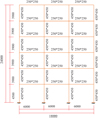 |
Fig. 2 Frame section size. |
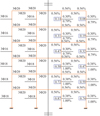 |
Fig. 3 Reinforcement diagram and axial compression ratio. |
Average strength of materials.
 |
Fig. 4 Correlation response spectrum curve. |
Seismic record selection results.
2.2 The application of NN in NSR simulation analysis
After completing the preparation of the sample set, in NSR analysis, the selection of nonlinear system models is first carried out. The study selected Nonlinear Auto Recursive Moving Average with exogenous input (NARMAX) with external input in equation (6).
 (6)
(6)
In equation (6), f(⋅) represents a nonlinear function. The input and output of the model were set to u(t) and y(t) respectively. t represents a discrete time scalar, and t = 0, 1, 2, ⋯. e ′ (t) means an unpredictable white noise with zero mean and finite variance. ny and nu represent the parameters of the NARMAX model. NARMAX provides a unified expression for implementable nonlinear systems. It has high approximation accuracy and fast convergence speed. NN was established in the study. Figure 4 shows the topology structure of the relevant model.
In Figure 5, the algorithm used is Error Back Propagation (BP) algorithm, which includes data forward propagation and error back propagation. u(t − 1) and u(t − 2) represents the model input at time t − 1 and t − 2, yˆ(t−1) and yˆ(t−2) represent the model output at time t − 1 and t − 2, and yˆ(t) represents the model output at time t. Input yˆ(t−1), yˆ(t−2), u(t − 1), and u(t − 2) into the model, and under the action of the BP algorithm, obtain yˆ(t). In the forward propagation section of the data, each neuron output of NN is defined in equation (7).
 (7)
(7)
In equation (7), netj represents the output of the j th neuron. In the previous story's i th node, its connection weight with the current story's j th node is Wij. f means the neuron activation function. The output of the previous story's i th neuron is Oi. The activation functions of neurons mainly include hyperbolic tangent and linear functions. Equation (8) represents the previous function.
 (8)
(8)
In equation (8), e represents the base of the natural logarithm. In the error backpropagation, the system error is defined during the training phase in equation (9).
 (9)
(9)
In equation (9), E represents the system error. The expected output of NN is ymn. The calculated output value of NN is omn. In BP, the gradient descent method is applied, and equation (10) is the relevant mathematical equation involved.
 (10)
(10)
In equation (10), η represents a value between 0 and 1, which is called the learning rate. The number of learning iterations is k. ΔWij represents the connection weight increment. In algorithm training, the algorithm output Hk+1 is corrected through the weight error function. The relevant mathematical formula for the weight correction of NN is equation (11).
 (11)
(11)
In equation (11), α, d, g, and β represent parameters. NN toolbox based on system identification can be used to identify dynamic nonlinear systems. Local modifications were made to the source program of the toolbox, and relevant NN was developed to make it suitable for SNSR simulation analysis. For the convenience of writing, NN is set to NSIN. In the program, equation (12) is the regression vector ϕ(t).
 (12)
(12)
In equation (12), the prediction error is ϵ(t). na and nb represent the parameters of the autoregressive moving average model. The time delay is nk, which is generally 1. The residual progression is nc. The analysis results of the research method were evaluated, and the selected evaluation indicators were time history curve, peak acceleration response, and relative energy. The duration of seismic motion is defined by the relative energy of the ground motion. For example, the time (t0.95−t0.05) from the moment when the ground motion energy reaches 5% of the total energy t0.05 to the moment when it reaches 95% of the total energy t0.95 is used as the definition of seismic motion duration, which is 90% energy duration. Through the time history curve, the nonlinear earthquake response under the time history can be more intuitively seen. Equation (13) represents the indicator in relative energy.
 (13)
(13)
In equation (13), the relative energy of the acceleration response simulation is Er. The relative acceleration value at moment t is at. In the acceleration response of discrete seismic motion, equation (14) is the corresponding Er.
 (14)
(14)
In equation (14), the time interval for the acceleration response is Δt. The acceleration response of the structure at moment i is Sai. Using these evaluation indicators, the errors in NN and elastic-plastic time history analysis results were analyzed.
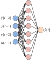 |
Fig. 5 Model topology. |
3 Analysis of SNSR based on NSIN
Based on artificial and natural earthquake records, the NSR of the designed frame structure under different characteristic period fields is simulated and analyzed using the research constructed NSIN. The obtained results were evaluated through time history curves, peak acceleration response, and other indicators, and the elastic-plastic time history analysis results were compared.
3.1 Simulation analysis of the response of artificial seismic records
NN model for NSR simulation was established. And artificial earthquake records from ACC1 to ACC9 and the corresponding acceleration response of the first floor of the plane frame were selected as the training sample set, with a duration of 30 s and a data volume of 9 in this sample set. The validation set consists of ACC10 and corresponding nonlinear acceleration responses from artificial seismic records, a data volume of 1 in this sample set, and the NSR of ACC11 to ACC20 was predicted. The elastic-plastic time history analysis was used as a comparison. Figure 5 shows the NSR simulation results of ACC11 in artificial seismic records.
Figure 6a shows the calculation results of the time history analysis under ACC11, and Figure 6b shows the calculation results of the research method under ACC11. Comparing Figures 6a and 6b and 6b, the trend of the curves is basically the same, and the fluctuation amplitude of the corresponding acceleration curve first gradually increases, then gradually decreases and approaches 0. Specifically, in Figure 6a, when the time is 7.5 s, the acceleration under time history analysis is 1.254 m/s2. At this moment, the acceleration under the research method in Figure 6b is 1.326 m/s2, which is 0.072 m/s2 smaller than the latter. When the time is 10 s, the acceleration under time history analysis is −0.876 m/s2, while the acceleration under the research method in Figure 6b is −0.706 m/s2. At this moment, the difference between the results calculated using the two methods is relatively small. When the time is 25 s, the acceleration corresponding to Figure 6a is slightly smaller than the research method, which has an acceleration of 0.17 s2. Therefore, the prediction effect of the research method is good. To further analyze the predictive performance of the research method, simulation analysis was conducted on the NSR of ACC12 in Figure 7.
Figure 7a shows the calculation results of the time history analysis under ACC12, and Figure 7b shows the calculation results of the research method under ACC12. Comparing two sub-graphs in Figure 6, the trend of changes in both curves is the same, with relatively large fluctuations in the curves between 5s and 20 s. In Figure 7a, at 12.5s, the acceleration under time history analysis is 1.742 m/s2, while the acceleration under the research method in Figure 7b is 1.349 m/s2, which is 0.393 m/s2 smaller than the latter. At 25 s, the calculation results of time history analysis and research methods were 1.715 m/s2 and 1.403 m/s2, respectively, with the former being 0.312 m/s2 smaller than the latter. Therefore, the prediction effect of the research method is good. The NSR prediction peak of the framework under the action of ACC11 to ACC20 was analyzed in Figure 8.
In Figure 8a, under the actions of different artificial earthquake records, the corresponding calculation results are different. Under the action of the same artificial earthquake record, there are certain differences in the calculation results of different methods, and the overall difference is relatively small. Under the action of ACC11, the time history analysis calculation result is 2.777 m/s2, which is 0.051 m/s2 larger than the research method calculation result, and the latter is 2.726 m/s2. Under the action of ACC18, the calculation results of time history analysis and research methods are 2.766 m/s2 and 2.758 m/s2, respectively. In Figure 8b, overall, the relative error of these two methods is relatively small under the action of different artificial seismic records. Among them, under the action of ACC16, the maximum relative error of these two methods is 11.28%, followed by ACC12, with a relative error of 8.86%. The minimum relative error of these two methods is 0.30%, which is 3.07% less than that under the action of ACC15. The prediction error of the research method is relatively small. Figure 9 analyzes the relative energy of nonlinear reactions under the actions of ACC11 and ACC12.
In the two sub-graphs of Figure 8, as time goes on, the relative energies of the nonlinear reaction under ACC11 and ACC12 gradually increase. In Figure 9a, when the time is 10 s, the relative energy of time history analysis is 3.898 m2/s, which is 0.263 m2/s higher than the research method, and the latter is 3.635 m2/s. When the time is 20 s, the relative energies of time history analysis and research methods are 8.063 m2/s and 7.349 m2/s, respectively. In Figure 9b, when the time is 30 s, the relative energy of the research method is 8.274 m2/s, which is 0.698 m2/s less than the time history analysis.
 |
Fig. 6 Correlation analysis results of ACC11. |
 |
Fig. 7 Correlation analysis results of ACC12. |
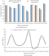 |
Fig. 8 Prediction peak results of nonlinear response of frames under the action of artificial earthquake records. |
 |
Fig. 9 Relative energy of nonlinear reactions. |
3.2 Response simulation analysis of natural seismic records
NN model constructed in the study was analyzed, with a site characteristic period of 0.30s. The training sample set used natural earthquake records and the corresponding acceleration response of the first floor of the plane frame, and a data volume of 19 in this sample set. The validation set included USA00623 and the corresponding nonlinear acceleration response, a data volume of 1 in this sample set and the NSR of USA00668 was predicted. Figure 10 shows the acceleration time history curve.
Figure 10a shows the calculation results of time history analysis under USA00668, and Figure 10b shows the calculation results of the research method under USA00668. Comparing the two sub-graphs in Figure 10, the trend of these two curves is the same. In Figure 10a, when the time is 12.5 s, the acceleration under time history analysis is 0.642 m/s2, while in Figure 10b, the acceleration under the research method is 0.378 m/s2, which is 0.264 m/s2 higher than the latter. When the time is 15.5 s, the calculation results of time history analysis and research methods are 0.658 m/s2 and 0.562 m/s2, respectively. Figure 11 analyzes the relative energies of nonlinear reactions under the actions of USA00668 and USA00869.
In these two sub-graphs of Figure 11, as time goes on, the relative energies of the nonlinear reaction under USA00668 and USA00869 gradually increase. In Figure 11a, when the time is 30 s, the relative energy of the time history analysis is 4.997 m2/s, which is 0.938 m2/s higher than the research method, and the latter is 4.059 m2/s. In Figure 11b, when the time is 20 s, the relative energy of the research method is 7.388 m2/s, which is 1.033 m2/s smaller than the time history analysis. Therefore, the research method performs well.
 |
Fig. 10 Correlation acceleration time history curve. |
 |
Fig. 11 The relative energy of nonlinear response under the action of natural earthquake records. |
3.3 Analysis of neural network prediction performance based on NARMAX model
Analyze the predictive performance of the research method, comparing the BP algorithm and Long Short Term Memory (LSTM) model. The training sample set and test dataset are the same as the dataset in Section 3.1. The prediction results recorded by ACC20 under different methods are shown in Table 3.
In Table 3, compared to other methods, research methods have higher accuracy and lower MAE values. In terms of accuracy, the accuracy of the research method is 95.68%, which is 16.65% higher than the BP algorithm and 8.23% higher than the LSTM model. It can be seen that the prediction performance of the research method is good.
Prediction results of different methods.
4 Conclusion
To understand the NSR situation of the structure, the research focuses on reinforced concrete frame structures. The experiment used NN as the research method and selected NN training samples. The results of elastic-plastic time history analysis were used as the output signal of the training samples. In the experiment, a suitable NN model was selected and NN simulation program was developed. On this basis, conduct NSR simulation. These results confirm that the research method has good predictive performance under the influence of artificial and natural earthquake records. Its prediction effect on the acceleration time history curve, acceleration response peak, and relative energy is good, and the error is relatively small compared to the calculation results of time history analysis. Under the action of ACC12, when the time is 12.5 s, the acceleration under the time history analysis is 1.742 m/s2, and the acceleration under the research method is 1.349 m/s2. The former is 0.393 m/s2 smaller than the latter. Under the action of ACC11, the time history analysis calculation result is 2.777 m/s2, which is 0.051 m/s2 larger than the research method calculation result, and the latter is 2.726 m/s2. Under the action of ACC11, when the time is 10 s, the relative energy of time history analysis is 3.898 m2/s, which is 0.263 m2/s higher than the research method, and the latter is 3.635 m2/s. Under the action of USA00668, when the time is 12.5 s, the acceleration under time history analysis is 0.642 m/s2, and the acceleration under the research method is 0.378 m/s2. Under the action of USA00869 for 20 s, the relative energy of the research method is 7.388 m2/s, which is 1.033 m2/s less than the time history analysis. Therefore, the application effect of the research method is good. There are still some shortcomings in the research, and it is recommended to conduct more complex NSR simulation analysis to expand the adaptability of the research method. In the future, research can be conducted in this direction.
5 Funding
The research is supported by Henan Province AHP-based small and medium-sized cost management enterprises digital transformation and upgrading, evaluation system research and construction (No. 2021SJGLX677).
References
- X. Guo, H. Lu, 3D simulation research on the damage of load-bearing structure of prefabricated building based on BIM model, Int. J. Crit. Infrastruct. 17, 170–186 (2021) [CrossRef] [Google Scholar]
- Y. Li, T. Shi, Y. Li, W. Bai, H. Lin, Damage of magnesium potassium phosphate cement under dry and wet cycles and sulfate attack, Constr. Build. Mater. 210, 111–117 (2019) [CrossRef] [Google Scholar]
- S. Yousefian Moghadam, M. Song, M.E. Mohammadi, B. Packard, A. Stavridis, B. Moaveni, R.L. Wood, Nonlinear dynamic tests of a reinforced concrete frame building at different damage levels, Earthq. Eng. Struct. Dyn. 49, 924–945 (2020) [CrossRef] [Google Scholar]
- A. Bayraktar, E. Hokelekli, Influences of earthquake input models on nonlinear seismic performances of minaret-foundation-soil interaction systems, Soil Dyn. Earthq. Eng. 139, 358–378 (2020) [Google Scholar]
- J. Zhang, K. Wei, L. Gao, S. Qin, Effect of V-shape canyon topography on seismic response of deep-water rigid-frame bridge based on simulated ground motions, Structures 33, 1077–1095 (2021) [CrossRef] [Google Scholar]
- Y. Zhang, X. Chen, X. Zhang, M. Ding, Z. Liu, Nonlinear response of the pile group foundation for lateral loads using pushover analysis, Earthq. Struct. 19, 273–286 (2020) [Google Scholar]
- D. Farahani, F. Behnamfar, H. Sayyadpour, Effect of pounding on nonlinear seismic response of torsionally coupled steel structures resting on flexible soil, Eng. Struct. 195, 243–262 (2019) [CrossRef] [Google Scholar]
- S. Cattari, B. Calderoni, I. Caliò, G. Camata, S. de Miranda, G. Magenes, G. Milani, A. Saetta, Nonlinear modeling of the seismic response of masonry structures: critical review and open issues towards engineering practice, Bull. Earthq. Eng. 20, 1939–1997 (2022) [CrossRef] [Google Scholar]
- Z. Alam, L. Sun, C. Zhang, Z. Su, B. Samali, Experimental and numerical investigation on the complex behavior of the localized seismic response in a multi-storey plan-asymmetric structure, Struct. Infrastruct. Eng. 17, 86–102 (2021) [CrossRef] [Google Scholar]
- C. Huang, Q. Gu, S. Huang, A practical method for seismic response analysis of nonlinear soil-structure interaction systems, Adv. Struct. Eng. 24, 2131–2147 (2021) [CrossRef] [Google Scholar]
- B. Zhang, Automatic seismic interval velocity building based on convolutional neural network and velocity spectrum, Geophys. Prospect. Pet. 60, 366–375 (2021) [Google Scholar]
- N. Nooshiri, C.J. Bean, T. Dahm, F. Grigoli, S. Kristjánsdóttir, A. Obermann, S. Wiemer, A. Multi-Branch, Multi-target neural network for rapid point-source inversion in a micro-seismic environment: examples from the Hengill geothermal field, Iceland, Geophys. J. Int. 229, 999–1016 (2021) [Google Scholar]
- F. Wang, S. Chen, Residual learning of deep convolutional neural network for seismic random noise attenuation, IEEE Geosci. Remote Sens. Lett. 16, 1314–1318 (2019) [CrossRef] [Google Scholar]
- H. Li, B.F. Spencer, Y. Lei, Y. Zhang, J. Mi, W. Liu, L. Liu, Detecting structural damage under unknown seismic excitation by deep convolutional neural network with wavelet-based transmissibility data, Struct. Health Monit. 20, 1583–1596 (2021) [CrossRef] [Google Scholar]
- Q. Xu, T. Zhang, J. Chen, J. Li, C. Li, The influence of reinforcement strengthening on seismic response and index correlation for high arch dams by endurance time analysis method, Structures, 32, 355–379 (2021) [CrossRef] [Google Scholar]
- F. Smarandache, Plithogeny, plithogenic set, logic, probability and statistics: a short review, J. Comput. Cognit. Eng. 1, 47–50 (2022) [Google Scholar]
Cite this article as: Feng Qin, Simulation analysis of structural nonlinear seismic response, Int. J. Simul. Multidisci. Des. Optim. 14, 18 (2023)
All Tables
All Figures
 |
Fig. 1 Plane layout and facade layout of the structure. |
| In the text | |
 |
Fig. 2 Frame section size. |
| In the text | |
 |
Fig. 3 Reinforcement diagram and axial compression ratio. |
| In the text | |
 |
Fig. 4 Correlation response spectrum curve. |
| In the text | |
 |
Fig. 5 Model topology. |
| In the text | |
 |
Fig. 6 Correlation analysis results of ACC11. |
| In the text | |
 |
Fig. 7 Correlation analysis results of ACC12. |
| In the text | |
 |
Fig. 8 Prediction peak results of nonlinear response of frames under the action of artificial earthquake records. |
| In the text | |
 |
Fig. 9 Relative energy of nonlinear reactions. |
| In the text | |
 |
Fig. 10 Correlation acceleration time history curve. |
| In the text | |
 |
Fig. 11 The relative energy of nonlinear response under the action of natural earthquake records. |
| In the text | |
Current usage metrics show cumulative count of Article Views (full-text article views including HTML views, PDF and ePub downloads, according to the available data) and Abstracts Views on Vision4Press platform.
Data correspond to usage on the plateform after 2015. The current usage metrics is available 48-96 hours after online publication and is updated daily on week days.
Initial download of the metrics may take a while.


