")
")
| Issue |
Int. J. Simul. Multidisci. Des. Optim.
Volume 10, 2019
|
|
|---|---|---|
| Article Number | A7 | |
| Number of page(s) | 7 | |
| DOI | https://doi.org/10.1051/smdo/2019004 | |
| Published online | 08 April 2019 | |
Research Article
Numerical modeling of shape memory alloy problem in presence of perturbation: application to Cu-Al-Zn-Mn specimen
1
Laboratory of Mechanics of Normandy (LMN), National Institute of Applied Sciences of Rouen,
Rouen, France
2
Laboratory of Mechanics, Modeling and Manufacturing (LA2MP), Mechanical Engineering Department, National School of Engineers of Sfax,
Sfax, Tunisia
3
Laboratory of System Engineering of Versailles, University of Versailles Saint Quentin In Yvelines,
Velizy, France
* e-mail: This email address is being protected from spambots. You need JavaScript enabled to view it.
Received:
1
October
2018
Accepted:
5
November
2018
Abstract
This paper proposes a methodology for taking into consideration uncertainties based on polynomial chaos (PC). The proposed approach is used in order to determine the response of Cu-Al-Zn-Mn shape memory alloy specimen with uncertainties associated to material parameters. The simulation results are obtained by PC method. The proposed method seems to be an efficient probabilistic tool. It is worth mentioning that PC approach is an interesting alternative for the parametric studies. This technique is more efficient compared to MC approach.
Key words: shape memory alloy specimen / material parameters / polynomial chaos method / uncertainty
© F. Abid et al., published by EDP Sciences, 2019
 This is an Open Access article distributed under the terms of the Creative Commons Attribution License (http://creativecommons.org/licenses/by/4.0), which permits unrestricted use, distribution, and reproduction in any medium, provided the original work is properly cited.
1 Introduction
In recent decades, smart technologies become of increasing interest in different engineering fields [1]. The purpose is to develop new and intelligent systems that can be integrated with actuators, sensors and micro controllers. Shape memory alloy (SMA) is a smart material that is successfully used in the achievement of such technologies [2]. SMA material becomes more and more used due to its interesting physical and mechanical properties compared to other materials. Such material is characterized by the ability to remember its original shape after deformation. In fact, SMA can generate high values of thermal-mechanical driving forces and can undergo reversible moderate deformations up to 8% under loading/thermal cycles. Such a specific behavior of SMA is because of the native capability to undergo reversible changes of the crystallographic structure that depends on the temperature and on the state of the stress. These changes are due to the martensitic transformations between the crystallographic more ordered parent phase, the austenite, and the crystallographic less ordered parent phase, the martenite [3]. Generally speaking, shape memory alloy is a major challenge for the researchers due to its intelligent characteristics. In fact, the main attractive features of this class of materials are the capabilities of: (1) recovering the original shape after large deformations induced by mechanical load (pseudo-elasticity) and (2) maintaining a deformed shape up to heat induced recovery of the original shape (shape memory effect) [4]. Due to its special behavior, SMA is easily integrated in systems without causing a high increase in volume or weight. Besides, such material is directly activated by temperature cycles or stress [5]. These characteristics allow the SMA to be used in a wide range of engineering applications such as biomechanics such as surgical tool and prostheses, aeronautics and automotive. The study of shape memory alloy does not integrate dispersion in the shape memory alloy parameters. They are considered as constant. However, such parameters are uncertain due to their experiment measurement. Several methods are proposed in the literature for considering uncertainties. Monte Carlo (MC) method is well-known in this field but it is often costly because of the great numbers of samples required in the aim to have a reasonable accuracy [5–7]. Polynomial chaos method is also presented in the literature as an attractive probabilistic method for considering uncertainties.
The capabilities of such a method are demonstrated in biological and environmental problem [12], in solving partial and ordinary differential equations [13], in dynamic systems [5] and in parameter estimation [14]. The main contribution of this communication is the study of the uncertainty of Cu-Al-Zn-Mn alloy. This communication is structured as follows: modeling of shape memory alloy specimen is presented in Section 2. One of the main contributions of this work, the MC and PC methodology are fully in Sections 3 and 4. Finally, numerical results of shape memory alloy problem and comments are made based on the methodology carried out in this communication in Section 5.
2 Modeling of Cu-Al-Zn-Mn alloy specimen
The considered model consists on a simple double notch specimen as shown in Figure 1. As a type of shape memory alloy, we choose the Cu-Al-Zn-Mn. The geometric characteristics of the studied specimen are the following: l = 6 mm, L = 70 mm and r = 2 mm. Numerical simulations of shape memory alloy response are performed using commercial software ANSYS.
Regarding the descritization of the specimen, 2D Plane 182 quadrilateral elements are used as shown in Figure 2. The 2D plane is formed by four node elements with four degrees of freedom at each node: 2 translations in the nodal x, y directions and 2 rotations in the nodal x, y. The values of the materiel parameters used in this model are given in Table 1.
These parameters are taken from literature [15] and are respectively: the Young's modulus E, the Poisson's ratio ν, the hardening parameter h, the reference temperature T0, the elastic limit R, the temperature scaling parameter β and the maximum transformation strain Ɛl.
In this problem, the bottom of the specimen (y = 0) cannot be moved. The applied loading path of the Cu-Al-Mn-Zn specimen is shown in Figure 3. The first step (AB) corresponds to the martensite variants orientation process. The second step (BC) corresponds to the thermal loading above the austenite finish temperature Af. Steps 1-2 and 2-3 correspond to the heating and cooling of the specimen. In this study, the room temperature and the heating level are fixed to 225 and 500 K.
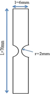 |
Fig. 1 2D diagram of the specimen. |
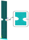 |
Fig. 2 ANSYS finite element model of the specimen. |
Material parameters.
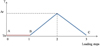 |
Fig. 3 Mechanical and thermal loading of the specimen. |
3 Monte Carlo (MC)
In this part, the Monte Carlo method is described. This method refers to any calculation technique using successive resolutions of a deterministic system incorporating uncertain parameters, which are modeled by random variables. It is a powerful mathematical tool, which is used, in a wide range
Of applications. An MC technique is used when the problem to be treated is complex for a resolution by analytic manner. It generates for all uncertain parameters and following their laws of probability and their correlations, random draws. For each draw, a set of parameters is obtained and a deterministic calculation, according to analytic or numerical models well defined, is operated [6]. This method can be applied to any system and the results are accurate. However, a reasonable accuracy needs a large number of draws. As a result, this method is expensive in term of computational time. Generally, the MC method is used as a reference method to validate the efficiency of others methods of uncertainty.
3.1 Algorithm implementation
The Monte Carlo method considers functions of the form:
 (1)
where M represents the model under consideration, U is the vector of uncertain input variables and X is the vector of the estimated outputs. In fact, the MC algorithm consists in five steps:
(1)
where M represents the model under consideration, U is the vector of uncertain input variables and X is the vector of the estimated outputs. In fact, the MC algorithm consists in five steps:
-
the probabilistic identification of the uncertain parameters of the studied system;
-
the sampling and the random generation of the achievements;
-
spread of the uncertainty of the data set obtained by step 2 into the model and the determination of the corresponding output set;
-
the estimation of the output distribution law;
-
the convergence analysis of the distribution of the model output.
4 Proposed method
Different methods are used in order to model the propagation of uncertainty. These techniques are classified in three categories: simulation technique, perturbation technique and spectral technique. Monte Carlo (MC) method is considered as a reference method in the calculation of system with uncertain parameters. The main problem of such a method comes from the high computational time which complicates the use of this technique. The perturbation technique considers the Taylor series development of the response around its mean. The main disadvantage of this method is the condition that ensures the convergence of these series. In fact, the variables must have low dispersion [8]. As a result, the method used in order to take into account uncertainty in this paper is the polynomial chaos (PC) method. The fundamental idea of PC, developed by Wiener [10] in 1938, is to separate the stochastic components of a random function and its deterministic components. In fact, the random process of interest is approximated by summing the orthogonal polynomial chaos of random independent variables [9]. The entire proposed methodology is described in the flowchart as shown in Figure 4. A brief mathematical review of this method is presented. For example, given any random variables Ui such as the displacement in a shape memory alloy system, we can write as follows [11]:
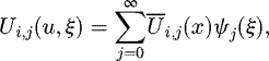 (2)
where ξ is a vector of standard normal random variables,
(2)
where ξ is a vector of standard normal random variables,  is the deterministic component and ψj(ξ) is the orthogonal polynomials such as Legendre, hermite, etc. The choice of the polynomial family is determined by the density distribution of the uncertain input parameter. As a result, a correspondence of the families of orthogonal polynomials and the families of probability laws is established. Because that a series expansion to infinity cannot be used in practice, the sum is truncated to an order Np in order to limit the number of terms to finite ones. The order Np depends on the dimension r of the polynomial chaos and its order p. We can write then:
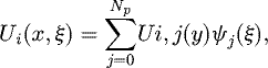 (3)with:
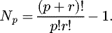 (4)
(4)
The calculation of the representation by the PC method requires the determination of Np + 1 stochastic components. The following step is to determine the PC coefficients by regression approach or spectral projection technique (NISP).
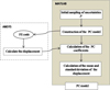 |
Fig. 4 Flowchart of the PC methodology. |
5 Numerical results and discussions
In this section, the analysis of the shape memory alloy specimen is performed with and without uncertainties.
5.1 Deterministic analysis
Figure 5 shows the shape memory alloy specimen during the steps (A-B) and (B-C) which are presented in Figure 3. Figure 6 gives the displacement as a function of applied temperature.
During the loading step, the temperature is kept constant at T = 225 K. For the step 2, the specimen is gradually heated to 500 K. After that, the temperature has returned to the room temperature. It seems that the specimen starts to move at a temperature equal to 285.5 K. This corresponds to the reverse transformation from martensite to austenite. The cooling allows it to return to a martensitic state.
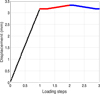 |
Fig. 5 Displacement during the steps 0-3. a: black line corresponding to mechanical load; b: red line corresponding to heating load; c: blue line corresponding to cooling load. |
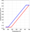 |
Fig. 6 Displacement as a function of heating. a: red line corresponding to heating load; b: blue line corresponding to cooling load. |
5.2 Sensitivity analysis
The purpose of this part is to study the sensitivity of the Cu-Al-Zn-Mn specimen response to input variables. Figure 7 represents the influence of the first set of physical parameters on the specimen considering a standard deviation of 20%. The set is formed by the Young's modulus E, the reference temperature T0, the temperature scaling parameter β and the maximum transformation strain Ɛl. By comparing these curves with the mean value curve, it can be clearly seen that these parameters have an influence on the behavior of the studied example. Figure 8 shows the displacement of the specimen considering the other set of the physical parameters: Poisson's ratio ν, the hardening parameter h and the elastic limit R. From Figure 8, we can conclude that these variables have a weak influence on the behavior of the specimen. In the next subsection, we will take into account the parameters that have an influence on the behavior of the studied specimen.
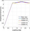 |
Fig. 7 Variables with influence in the displacement. |
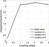 |
Fig. 8 Variables with non influence in the displacement. |
5.3 Probabilistic analysis
In this part, the static behavior of Cu-Al-Zn-Mn specimen is investigated using polynomial chaos (PC) approach. The PC results are compared with the Monte Carlo (MC) method. The material parameters of such a studied system are summarized in Table 1. Uniform probability distribution is treated in order to describe the random parameters. In this case, the Legendre polynomials are the best used to deal with uniform uncertainties. They are calculated using the recurrence relation as mentioned in the equation:
 (5)
(5)
Numerical results are presented for the formulation derived in Section 3. The material variables of the Cu-Al-Zn-Mn specimen that influence in the displacement are respectively: the Young's modulus E, the temperature scaling parameter β, the reference temperature T0 and the maximum transformation strain Ɛl. These variables are supposed to be random and they are defined as shown in Table 2. The parameters are chosen to be random following a uniform distribution around their normal values ± 20%.
Using the Monte Carlo approach consists on creating a grid of numerical values from the certain parameters and calculating the quantity of interest. The quantity of interest is analyzed for 500 simulations. Figure 9 represents the distribution of the input variables (E, β, T0, Ɛl) in the case of uniform distribution. Figures 10 and 11 present the evolution of the displacement as a function of loading steps by two stochastic approaches MC and PC in the case of 4 uncertain parameters and for two values of PC orders.
The mean value and the standard deviation of the displacement of the specimen are calculated by polynomial chaos approach. The obtained results are compared with those given from MC simulations for 500 simulations. Figures 10 and 11 show the mean value and the standard deviation of the displacement of the specimen in the case of p = 1 and p = 3. It can be seen from these figures that as p increases, the result seems to become better. For p = 3, the displacement of the specimen matches with the MC simulations results. These figures show that the obtained solutions are around the Monte Carlo simulation which is the reference solution. Besides, one can notice that the computational time is considerably reduced. Table 3 presents a summary of the two stochastic methods used in this example.
It is worth mentioning that the Monte Carlo approach is a well-known technique used in order to solve complex system with uncertainties. To have a reasonable accuracy, this method requires a great number of samples. In this paper, 500 of sampling of 4 input variables are calculated and then the problem is solved for each sample of input variables.
However, this approach has a poor convergence for the mean and the standard deviation of the solution. Thus, it requires a large number of samples to have a good precision. The PC method is used as an alternative to deal with the uncertainty, quantification. Such a method is more efficient compared to MC method.
Characteristic of uncertain parameters.
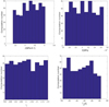 |
Fig. 9 Probability distribution of the inputs. a: the Young's modulus E; b: the temperature scaling parameter β; c: the reference temperature T0; d: the maximum transformation strain Ɛl. |
 |
Fig. 10 Mean value of the displacement. |
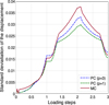 |
Fig. 11 Standard deviation of the displacement. |
Summary results of the displacement.
6 Conclusion
In this work, the Monte Carlo method and the PC approach were coupled to finite element solutions discussed above in order to calculate the displacement of the Cu-Al-Zn-Mn specimen. The response of such a material is coupled to probabilistic approaches when material parameters present uncertainties. Results using PC are compared with MC method. Convergence was verified with comparisons against solution from MC simulations. The main results of the present study demonstrate that the PC method may be an effective alternative of MC simulations. As regard efficiency, the PC based simulation is computationally less expensive compared to MC in order to generate solutions. A future track of this work is to apply optimization under uncertainty in complex system formed by shape memory alloy. Further work in this context is in progress.
Acknowledgments
The present research work has been supported by the laboratory of mechanics of normandy (LMN), INSA Rouen and the laboratory of mechanics, modeling and manufacturing (LA2MP), ENI Sfax. The authors gratefully acknowledge then support of these institutions
References
- D.C. Lagoudas (Ed.), Shape memory alloys: Modeling and engineering applications (Springer-Verlag, 2008) [Google Scholar]
- T. Merzouki, A. Duval, T.B. Zineb, Finite element analysis of a shape memory alloy actuator for a micropump, Simul. Model. Pract. Theory 27, 112 (2012) [CrossRef] [Google Scholar]
- P. Bisegna, F. Caselli, S. Marfia, E. Sacco, A new SMA shell element based on the corotational formulation, Comput. Mech. 54(5), 1315 (2014) [CrossRef] [Google Scholar]
- A. Alipour, M. Kadkhodaei, A. Ghaei, Finite element simulation of shape memory alloy wires using a user material subroutine: Parametric study on heating rate, conductivity, and heat convection, J. Intell. Mater. Syst. Struct. 26(5), 554 (2015) [CrossRef] [Google Scholar]
- A. Guerine, A. El Hami, L. Walha, T. Fakhfakh, M. Haddar, Dynamic response of a spur gear system with uncertain parameters, J. Theor. Appl. Mech. 54(3), 1039 (2016) [CrossRef] [Google Scholar]
- K. Dammak, A. El Hami, S. Koubaa, L. Walha, M. Haddar, Reliability based design optimization of coupled acoustic-structure system using generalized polynomial chaos, Int. J. Mech. Sci. 134, 75 (2017) [CrossRef] [Google Scholar]
- K. Dammak, S. Koubaa, A. El Hami, L. Walha, M. Haddar, Numerical modelling of vibro-acoustic problem in presence of uncertainty: Application to a vehicle cabin, Appl. Acoust. 144, 113 (2019) [CrossRef] [Google Scholar]
- M. Beyaoui, M. Tounsi, K. Abboudi, N. Feki, L. Walha, M. Haddar, Dynamic behaviour of a wind turbine gear system with uncertainties, Comptes Rendus Méc. 344(6), 375 (2016) [Google Scholar]
- K. Sepahvand, M. Scheffler, S. Marburg, Uncertainty quantification in natural frequencies and radiated acoustic power of composite plates: Analytical and experimental investigation, Appl. Acoust. 87, 23 (2015) [CrossRef] [Google Scholar]
- N. Wiener, The homogeneous chaos, Am. J. Math. 60(4), 897 (1938) [CrossRef] [MathSciNet] [Google Scholar]
- L. Nechak, S. Berger, E. Aubry, Robust analysis of uncertain dynamic systems: Combination of the centre manifold and polynomial chaos theories, WSEAS Trans. Syst. 9(4), 386 (2010) [Google Scholar]
- S.S. Isukapalli, A. Roy, P.G. Georgopoulos, Stochastic response surface methods (SRSMs) for uncertainty propagation: Application to environmental and biological systems, Risk Anal. 18(3), 351 (1998) [CrossRef] [Google Scholar]
- M.M.R. Williams, Polynomial chaos functions and stochastic differential equations, Ann. Nucl. Energy 33(9), 774 (2006) [CrossRef] [Google Scholar]
- G. Saad, R. Ghanem, S. Masri, Robust system identification of strongly non-linear dynamics using a polynomial chaos-based sequential data assimilation technique, in: 48th AIAA/ASME/ASCE/AHS/ASC Structures, Structural Dynamics, and Materials Conference, 2007, p. 2211 [Google Scholar]
- N. Motte, A study to evaluate non-uniform phase maps in shape memory alloys using finite element method, Doctoral dissertation, Virginia Commonwealth University, 2015 [Google Scholar]
Cite this article as: Fatma Abid, Abdelkhalak Elhami, Tarek Merzouki, Hassen Trabelsi, Lassaad Walha, Mohamed Haddar, Numerical modeling of shape memory alloy problem in presence of perturbation: application to Cu-Al-Zn-Mn specimen, Int. J. Simul. Multidisci. Des. Optim. 10, A7 (2019)
All Tables
All Figures
|
Fig. 1 2D diagram of the specimen. |
| In the text | |
|
Fig. 2 ANSYS finite element model of the specimen. |
| In the text | |
|
Fig. 3 Mechanical and thermal loading of the specimen. |
| In the text | |
|
Fig. 4 Flowchart of the PC methodology. |
| In the text | |
|
Fig. 5 Displacement during the steps 0-3. a: black line corresponding to mechanical load; b: red line corresponding to heating load; c: blue line corresponding to cooling load. |
| In the text | |
|
Fig. 6 Displacement as a function of heating. a: red line corresponding to heating load; b: blue line corresponding to cooling load. |
| In the text | |
|
Fig. 7 Variables with influence in the displacement. |
| In the text | |
|
Fig. 8 Variables with non influence in the displacement. |
| In the text | |
|
Fig. 9 Probability distribution of the inputs. a: the Young's modulus E; b: the temperature scaling parameter β; c: the reference temperature T0; d: the maximum transformation strain Ɛl. |
| In the text | |
|
Fig. 10 Mean value of the displacement. |
| In the text | |
|
Fig. 11 Standard deviation of the displacement. |
| In the text | |
Current usage metrics show cumulative count of Article Views (full-text article views including HTML views, PDF and ePub downloads, according to the available data) and Abstracts Views on Vision4Press platform.
Data correspond to usage on the plateform after 2015. The current usage metrics is available 48-96 hours after online publication and is updated daily on week days.
Initial download of the metrics may take a while.