")
")
| Issue |
Int. J. Simul. Multidisci. Des. Optim.
Volume 16, 2025
|
|
|---|---|---|
| Article Number | 1 | |
| Number of page(s) | 17 | |
| DOI | https://doi.org/10.1051/smdo/2024021 | |
| Published online | 07 January 2025 | |
Research Article
Decision-making in clinical diagnostic for brain tumor detection based on advanced machine learning algorithm
School of Information Engineering, Hunan University of Science and Engineering, Yongzhou 425199, Hunan, China
* e-mail: This email address is being protected from spambots. You need JavaScript enabled to view it.
Received:
27
June
2024
Accepted:
17
September
2024
Abstract
Brain tumors, abnormal growths in the brain or spinal canal, can be benign or malignant, causing symptoms like headaches, seizures, and cognitive decline by disrupting brain function. Therefore, developing reliable predictive models for diagnosis and prognosis is crucial. In this paper, the prediction of brain tumors is made using machine learning models enhanced by an optimizer, namely Escaping Bird Search Optimization. Optimized models incorporate Ada Boost Classifier (ADEB), Gaussian Process Classifier (GPEB), and Support Vector Classifier (SVC) which, after being tested on a few databases, were named ADEB, SVEB, and GPEB, respectively, and their predictive power was assessed. The best single model performance overall on all databases is the SVC with an average accuracy of 0.981, while among enhanced models, the optimized model, called SVEB, using SVC, attained the highest accuracy for all models and reached as high as 0.990. These findings underscore the role of optimization techniques and demonstrate the effectiveness of machine learning in predicting brain cancers. The improved performance of the enhanced SVC model, SVEB, suggests it could offer a reliable approach for accurate brain tumor prediction. Enhanced patient outcomes and early diagnosis could be an implication of this in the field of neuro-oncology.
Key words: Brain tumor classification / machine learning / Ada boost classifier / Gaussian process classifier / support vector classifier
© T. Huang et al., Published by EDP Sciences, 2025
 This is an Open Access article distributed under the terms of the Creative Commons Attribution License (https://creativecommons.org/licenses/by/4.0), which permits unrestricted use, distribution, and reproduction in any medium, provided the original work is properly cited.
1 Introduction
The human brain is a complex interconnection of neurons and synapses. It acts as the central nervous system to coordinate various physiological and cognitive tasks essential in life. Like other major organs, it can be subject to various degenerative diseases. One particularly serious problem pertains to that of tumors of the brain. Brain tumors are a heterogeneous group of neoplastic entities, diverging in their clinical relevance. They are characterized by the abnormal proliferation of cells inside the brain or central spinal canal. These tumors represent a heterogeneous group, including benign growths and malignant malignancies. They may arise from many types of neural cells or from the metastasis of cancerous cells that have developed in other areas of the body [1]. The diagnosis and management strategy for brain tumors appropriately requires the etiological factors, clinical symptoms, and therapeutic techniques involved task that calls for a complex interplay of neurological structures and functions. Such insight not only helps medical professionals make decisions about diagnosis and treatment but also has significant ramifications for improving patient outcomes and the quality of life when dealing with this powerful pathogenic entity [2].
1.1 Causes of brain tumors
There are some known risk factors for brain tumors, although the exact cause remains largely unknown. These include exposure to ionizing radiation, genetic predisposition, impairment of the immune system, and some genetic disorders like neurofibromatosis and Li-Fraumeni syndrome. Furthermore, several reports indicate that exposure to electromagnetic fields and certain environmental chemicals may be associated with brain malignancies; however, further investigation is still required to verify the results [3,4].
1.2 Signs and symptoms
These can vary, depending on size, location, and the tumor's growth rate. Common signs and symptoms include persistent headache, seizures, a change in eyesight, difficulty speaking, impaired coordination, cognitive deficits, and personality changes [5]. Symptomatic presentation is not unique, as these signs and symptoms can theoretically also arise from some other neurological conditions. As such, all symptoms that are irritating or persistent should be seen by a medical professional [6].
1.3 Diagnostic techniques
Diagnosis of brain tumors is often made by using an approach that includes accurate neurological examination, biopsy of the tissue for histopathology, and neuroimaging techniques like magnetic resonance imaging (MRI) [7] or computed tomography (CT) [8] scans. These diagnostic studies outline the critical details on site, size, and histological attributes of the tumor that are highly pertinent in the formulation of an individualized treatment approach that can delay the disease's progression and thus help improve outcomes. Based on putting together all those diagnostic insights, healthcare practitioners can thus navigate effectively through the underlying management complexity in brain tumors. This allows precision medicine approaches to be instituted that are tailored to meet the individual patient's needs [9].
1.4 Treatment options
The management of brain tumors will depend on several factors, which include the size of the tumor, anatomic location, histology, and overall health of the individual. The therapeutic techniques range from targeted molecular medicines, immunotherapeutic approaches, radiation therapy, chemotherapy, and surgical resection [10]. Often, it is an overall approach that includes multiple modalities to best achieve success in treatment and hinder the disease's further progression. The goals of treatment include eradication or shrinking of the tumor, alleviation of symptoms, prevention of recurrence, and preservation of neurological integrity. In brain tumor management, the medical fraternity tries to customize the management plans according to the individual profile of the case for maximum therapeutic benefit and a better long-term prognosis [9,11].
1.5 Surgery
The treatments for accessible brain tumors start with surgery, aiming at maximal safe removal of the tumor. The surgical goal is the maximal tumor removal in order to minimize injury to surrounding normal brain tissue. However, the location of the tumor and proximity to critical neurovascular structures may impose limitations that prevent total removal. Under these conditions, the main goals of surgical approaches are to preserve cerebral function and to minimize post-surgical sequelae [12,13]. The fine balance reached between tumor removal aggressively and preservation of neurological function underlines the need for personalized strategies that are based on precise anatomical considerations and individual patient factors [14]. To this, this approach underlines the multifaceted nature of decision-making that forms a basis of neurosurgical management of brain tumors [15].
1.6 Radiation therapy
High-energy beams in radiation therapy are utilized to target and destroy malignant cells. It can be given internally through brachytherapy or externally through external beam radiation therapy. It may serve as a first line of treatment for inoperable cancers, additional treatment following surgery, and for alleviating symptoms and reducing tumor growth [16].
1.7 Chemotherapy
In chemotherapy, drugs are utilized that either destroy or inhibit the expansion of cancer cells. Chemotherapy is either used alone or in conjunction with other treatments, and it is given either orally or intravenously. When the other treatments cannot control the aggressive or recurrent brain tumor, chemotherapy is commonly used [17].
1.8 Targeted drug therapy
Targeted drug treatment is more efficient and less harmful than general chemotherapy. It acts by attempting to block the activity of specific molecules or pathways participating in tumor growth and development. Examples of targeted therapies include drugs interfering with angiogenesis, that is, the creation of new vessels, signal transduction inhibitors, or immunotherapies. They are based on the molecular features of the tumor [18–20].
1.9 Immunotherapy
Due to immunotherapy, the body's immune system identifies and attacks cancerous cells. It has appeared promising for specific kinds of brain tumors that demonstrate an enormous amount of immune cell infiltration [21]. Under immunotherapies, checkpoint inhibitors and therapeutic vaccinations, and adoptive cell transfer therapies fall in [22].
1.10 Clinical trials
Clinical trials also contribute to the elaboration of new therapeutic modalities and provide knowledge about brain tumors. Such studies may involve the evaluation of new therapeutic options regarding efficacy and toxicity and may offer new choices for patients who have exhausted their possibilities of conventional care. The participation in clinical trials offers the chance to get new drugs and contributes to the oncological knowledge base [23].
1.11 Role of machine learning
This sub-area of AI, in some ways called “machine learning” (ML), focuses on the elaboration of statistical frameworks which will permit computers to learn from data and make decisions or predictions without being explicitly programmed [24]. More particularly, in the context of ML, it is based on pattern and relationship searching in databases that are later applied to predict or determine what actions to undertake with new data. It normally comprises data preparation, feature selection or extraction, model training, and model testing [25]. The Ada Boost Classifier (ADA), Gaussian Process Classifier (GPC), and Support Vector Classifier (SVC) are three main machine learning models that could help in finding whether a patient has a brain tumor or not. ADA displays an ensemble learning method combining multiple weak classifiers to achieve a robust predictive model [26]. Tumor detection and segmentation can be done, therefore, with high precision by the efficient integration of various considered imaging data to enhance classification accuracy from either CT or MRI images [27]. Using its probabilistic architecture, GPC may strongly predict the outcome through spatial heterogeneity characterization within tumor regions and quantification of the uncertainty in tumor border delineation. It can further be extended to different image modalities. In finding the hyperplane that optimally separates tumors from non-tumor occurrences in feature space, SVC performs excellent jobs in class separation and hence enables accurate prediction within intricate imaging databases. These machine learning models provide physicians with diagnostic tools that can allow early tumor detection and make appropriate informed therapeutic decisions on improvement in neuro-oncology patient outcomes.
2 Study techniques and techniques
2.1 Data collection
The database on brain tumor features analyzed is a tabular arrangement of numerical features supposed to describe the radiographic features in images of brain tumors. This database contains a carefully preselected subset of features that fall into two categories: first-order statistical measurements and second-order texture descriptors. The first-order features represent the main characteristics of the distributions of pixel intensities and, indeed, encapsulate information on mean, variance, standard deviation, skewness, and kurtosis. This feature provides information about central tendency, dispersion, and form of the intensity distribution in images. In contrast, second-order features tap into the textural subtleties available in images to uncover spatial relationships and patterns beyond pixel-intensity data. These are contrast, energy, angular second moment, entropy, homogeneity, dissimilarity, correlation, and coarseness. Each of these measures gives a different insight into the spatial heterogeneity and structural complexity in these images. Hence, the binary target variable is annotated, which is represented by the “Class” column in this database. 1 displays the presence of a brain tumor, while 0 no tumor in an image. Each data entry also has an image ID to trace and link easily from source original image data. The well-structured nature of this database displays the base of computational analyses and machine learning efforts invested in underpinning radiomic signatures and discriminant features that characterize the pathology of brain tumors, with views toward the improvement of both clinical diagnosis and therapeutic intervention strategies in neurooncology.
Clear insight into how each input parameter influences the final results may be achieved by analyzing (Fig. 1). These are emphasized through the use of a color-coded scheme that highlights the different magnitudes of these various parameters' effects. The observations of particular significance show that measures such as mean and correlation influence insignificantly small values zero, insinuating their negative impact on the results. In contrast to this, the dissimilarity parameter has demonstrated a strong positive effect that almost touches 0.6, showing the immense value this parameter holds on the results. Moreover, those measures that significantly contribute to the observed effects also include variance, standard deviation, skewness, kurtosis, and contrast. Their positive effects range from 0.2 to 0.4. In contrast, while defining negative effects, it is worth noting that factors such as energy and homogeneity exhibit noticeably bad effects close to one, indicating their profoundly negative impact. Furthermore, even though they have negative effects, factors like ASM and Entropy exhibit comparatively smaller magnitudes than their previously described equivalents, indicating subtle differences in their influence on the final results. Figure 2 presents the histogram along with the normal distribution curve for both the input and output variables. This visualization allows for a clear comparison between the actual distribution of the data and the idealized normal distribution, providing insights into the underlying frameworks and variability in the database.
 |
Fig. 1 The plot illustrates the correlation between the input and output. |
 |
Fig. 2 The histogram-normal distribution plot for inputs and output. |
 |
Fig. 2 (Continued). |
2.2 Adaptive-boost learning (ADAC)
Versatile lift learning, or AdaBoost, [28], has been widely used in AI to create powerful classifiers from a small number of weak sub-classifiers (such as binary trees and SVM). Its effectiveness in preventing over-fitting problems has also been fully confirmed. As of right now, the preparation strategy is fully advancing and makes use of AdaBoost. Using a weighted irregular inspection method, the sub-classifiers {An (.) |n = 1, 2, … , N} undergo successive preparation. For each An(.) to be prepared, a subset of tests is chosen from the entire database.
 (1)
(1)
where the first databases, sample weights, and sampling ratio, respectively, are denoted by X, Wn, and Y, and φ stands for the testing protocol suggested by Pavlos et al. [29]. For every case, the weight Wn is ascertained as:
 (2)
(2)
Zn, which displays the total count of samples in the original database, and N, the sum of all weights used to normalize the weights between (0,1), reflect the predicted label from the previously trained classifier An-1(∙). A negative logit function is used to calculate the coefficient γn-1:
 (3)
(3)
where the weighted error rate of the classifier An-1(∙) is represented by ρn-1
 (4)
(4)
when ρn-1 is less than 0.5, it displays that γn-1 is not equal to zero. The definition of the sign function represented by τ(∙) in (2) is
 (5)
(5)
In equation (2), if γn-1 > 0 and y ≠ ŷ, then it's larger than 1. The sample that An-1(∙) mistakenly identified then accumulates weight, increasing the likelihood that it will be chosen for An-1(∙) training. This is the factor of scaling eγn−1·τ(yi,ŷi). Figure 3 presents the flowchart of the ADAC.
 |
Fig. 3 The flowchart of the ADAC. |
2.3 Gaussian process classifier (GPC)
GPC is a nonparametric probabilistic classification classifier based on Gaussian process regression [30]. When using GPC, the likelihood that the input data would fall into a particular class is correlated monotonically with the value of an underlying latent function attached to the data. Examine a database that includes observations labeled y = (y1, y2,..., yN) and x = (x1, x2,..., xN). In this scenario, xt = (xt,1, xt,2, … , xt,p) T displays the vector of w inputs at time t, and yt displays the appropriate binary response, that is, yt ϵ{1,-1} for t =1,…, N. Providing the notion of an unknown “latent function, ft,” is more convenient to simplify the response distribution yt representation.
 (6)
(6)
The link function is s, and the coefficient vector is C in the example  . This signifies that the probability of yt = 1 is determined by a nonlinear function, that is, the product of the linear combination of the input data Xt. For instance, the following is one approach to think of a logistic framework for a binary goal:
 (7)
(7)
The link function is expressed as s (z) = (1 + exp(− z)) −1.
Given inputs X1, X2, · · · , XN, let the latent functions f = [f (X1) , ·· · , f (XN)] follow a multivariate Gaussian distribution. A Gaussian process's mean and covariance functions give all of its characteristics. Said another way,
 (8)
(8)
The N×N covariance matrix of f in this instance is represented by V(X, X′), and Vi,j is the (i, j)-th element; that is, V(Xi, Xj). [μ (X1) , … , μ (XN)] is the representation of the mean vector µ(X). Note that for the sake of this article, µ(X) is assumed to be zero, i.e., µ(X) = 0.
 (9)
(9)
The covariance function, V(X, X′), which influences how responses at one input, Xi, are affected by responses at another input, Xj, defines the link between latent variables. Many kernel functions, including the ARD exponential kernel function (Eq. 10), shape the covariance function K (· ,·). These kernels provide unique smoothness and structural features that allow modification to better capture complex relationships between latent variables.
 (10)
(10)
The hyper-parameters  denote the unique length scales, while the scale parameter
  displays the importance of specific areas. In short, the characteristic length scale displays the distance between input values Xi, or the range of values within which response values are uncorrelated. In the testing or prediction database, X* stand for the input data. It is possible to obtain the latent value representing the testing data, represented by the symbol f* and written as X*‵C. Eq. (11) can be used to derive the posterior probabilistic forecast of the probability π* = p (y* = 1).
 (11)
(11)
where
 (12)
(12)
A formula for calculating the probability p(f | X, Y) can be found in equation (13).
 (13)
(13)
The symbol p(f |X) depicts the Gaussian prior distribution of f, CP(0,V(X, X′). The normalization term Z, defined as  , displays the marginal likelihood. For binary classification, a probit likelihood is adopted, where the term p(yi | fi) displays the density function of a conventional normal distribution.
Gaussian process techniques often have an O(n3) processing cost because of the inversion of the covariance matrix. To reduce this complexity, however, several sparse approximation techniques have been developed, including variational inference (VI), Laplace approximation (LA), expectation propagation (EP), and Markov Chain Monte Carlo (MCMC). See [31] to learn more about these approximation techniques for GPC. Moreover, [32] offers an in-depth examination of many sparse approximation techniques. Throughout the research, the Expectation Propagation (EP) approach from [33] is used to approximate the Gaussian posterior distribution given in equation (11). The posterior probability function p(f | X, Y), as provided by equation (14), can be approximated.
 (14)
(14)
The site parameters are fundamental components of the normalized Gaussian distribution denoted by the letter N. They are represented by the notations ũi and σ˜i2.
 (15)
(15)
and
 (16)
(16)
The elements of the diagonal matrix  are
are  and
and
 .
.
By equations (12) and (14), equation (17) provides the Gaussian approximation to the posterior distribution given in equation (11).
 (17)
(17)
Here, V* = V (X, X*).
2.4 Support vector classification (SVC)
Using support vector machines, SVC is an ML technique [34] that reduces risk by making non-linear changes to independent variables. The objective is to maximize margins, hyperplane distances, and training samples closest to each class while minimizing classification errors and constructing the best possible hyperplane to divide groups [35]. Equations are then used to present the principal model [36].
 (18)
(18)
 (19)
(19)
 (20)
(20)
Using a nonlinear transformation function ∂ (xi), an explanatory variable xi representing each observation is transformed into a higher-dimensional space. This new domain is represented by the feature space, and the weight vector associated with the independent variables is denoted by Pv. Additionally, the regularization parameter Csvc and the bias term b is introduced. Slack variables indicate the separation between an observation (i) and the edge or margin of its class. They are denoted by the symbol Δi.
An optimization procedure to identify the optimal hyperplane in this high-dimensional space that maximizes the margin is initiated by equation (21). This is done to reduce both the number of cases that are wrongly classified and the norm of the weight vector. The class labels applied to each sample ultimately indicate the classes that correlate with it.
 (21)
(21)
The dual version of the framework is based on sample counts, whereas the original framework's scale is determined by the problem's complexity. Therefore, when dimensionality is high enough, handling the dual model is desirable, as demonstrated by equations (22)–(24).
 (22)
(22)
 (23)
(23)
 (24)
(24)
The function known as 𝒦 (xi, xj) is responsible for mapping pairs of data points to feature space. There are several Kernel functions accessible, but they must be positive semi-definite, symmetric, polynomial, radial basis, and sigmoidal. Previous research displays that the radial basis Kernel function referred to as equation (25) is useful, especially for categorization applications [37]. Employing this function in methodology, wherein γ functions as a hyperparameter denoting the inverse range of effect of data points labeled with support vectors [38].
 (25)
(25)
Equation (26), which may be used to solve the model, provides estimates for the weights and bias factor as well as forecasts for more samples.
 (26)
(26)
2.5 Escaping bird search optimization (EBSO)
EBS is a population-based framework in which pairs of artificial birds function as search agents to assess the design space. In each randomly chosen pair from the population, one bird with lower fitness becomes the prey (escaping bird), and the other becomes the predator [39], [40]. The position of a synthetic bird in the investigation domain is in line with a design vector that changes as the bird flies. The bird's agility is affected by its body area, wing beat rate, and speed [41]. In the current numerical simulation, the maneuver_power of the ith artificial bird, MPi, is defined by equation (27);
 (27)
(27)
By deducting the prior location from the present position of the bird, Wi, the velocity vector, is obtained, from which the maneuver_power of the ith bird is computed. is the formula for calculating the square root of the sum of the squared elements of Wi, which yields the norm of Vi. To simulate the impact of wing beat-rate fluctuation on maneuver_power, the parameter ω is included, randomly varying between 0 and 2. The normalized relation body factor ri is expressed to indicate the effect of the bird's body area (cost) in modeling.
 (28)
(28)
The phrase above can be used to compute the cost of the ith agent represented as Gi. Here, Gmax and Gmin stand for the largest and minimum costs, respectively, among the current population. A minuscule constant, ϵ, is inserted to prevent division by zero. Furthermore, as the predator and prey, respectively, the Attacking Bird (AB) and Escaping Bird (EB) maneuverability is taken into account while calculating the Escaping Rate (ER). Equation (29) is utilized to ascertain the ER.
 (29)
(29)
Both the escaping bird and the attacking bird's maneuvering abilities are denoted by the labels MPEB and MPAB, respectively. When a bird of prey engages in vertical maneuvering, it chooses a destination that is opposite to the predator. The artificial flight used to replicate this is as follows:
 (30)
(30)
The situations of the fleeing bird and the attacking bird are indicated by XEB and XAB, respectively. A uniformly distributed variable, s, is created at random from 0 to 1. Equation (29) is used to determine the ER. To find the opposite of a given vector, use the Op(.) function, which is displayed as the vector's opposite in the design space [42].
 (31)
(31)
The artificial prey will choose a lateral movement, which involves shifting direction from the current course if the ER is tiny in size. A randomly generated position vector is utilized as a switch to numerically replicate this:
 (32)
(32)
XL and XU are the vectors that reflect the lower and upper boundaries of the design variables, respectively. In vector R, random values from 0 to 1 are contained; the τ symbol displays the element-wise product. During flight, the predator's primary goal is to locate its prey. However, this flight has another direction added by the current simulation: it flies in the direction of XGbest, which is the worldwide average of all prey experiences so far. Thus, the movement of the predator is represented as:
 (33)
(33)
within the range of 0 to 1, the random values s1 and s2 are created individually. The Capturing Rate (CR) is displayed as:
 (34)
(34)
The capturing rate falls toward zero when the escape rate is changed, and vice versa, demonstrating how CR and ER work in tandem. Predator and prey effects are included in equation (32) for difficulties involving the air. Vector-sum position updating is used in equation (33), which is different from popular meta-heuristic techniques like PSO. But unlike PSO, which ignores cognitive and inertial aspects, the algorithm, EBS, only considers an adaptation coefficient, CR. In addition, the last term in equation (33) does not scale by a constant proportion. Following the stages below, the suggested algorithm advances by mimicking artificial predator-prey maneuvers:
Step 1: Determine each ith bird's position inside the bottom and upper boundaries of the design variables. Assign each artificial bird a position at random to create a population of M birds. Using the following equation (35):
 (35)
(35)
The right-side parameters have been established by the equation in equation (32). The cost function for each bird will then be computed, and their velocities will be set to 0. Step 3 will distinguish between the prey and predator birds that make up the original population.
Step 2: Use equation (27) to determine the maneuver_power value for each bird, accounting for the normalization of cost values derived from equation (28).
Step 3: Proceed with running the main loop until the given closure condition is filled in:
For every i between 1 and M:
Select a bird at random from the population at the position ith and couple it with another bird.
Choose the best bird to be the AB and the other bird to be the EB.
For every pair (AB, EB), carry out the following actions:
Use equations (27)–(29) and (34) to determine the MP, ER, and CR for the current pair.
To create a potential solution for AB, use equation (33).
Calculate the candidate solution's cost,
 .
.Replace XAB with
 if
if  is less expensive than XAB.
When the total number of fitness function evaluations (NFE), also known as NFEmax, reaches a specified maximum value, and ends the main loop.
Next, generate a feasible EB solution through the application of either level-turning (Eq. (32)) or vertical-maneuvering (Eq. (29)). Switch between these evasion strategies following the relationship provided:
 (36)
(36)
Take the subsequent actions for EB:
Analyze the candidate solution's cost,
 .
.Replace XEB with
 (greedy selection) if
  is less expensive than XEB.
When NFE approaches NFEmax, immediately end the main loop.
Update XGbest.
If NFE < NFEmax and i =M, go back to Step 3. If not, close the loop and move on to Step 4.
Step 4: Declare the modified XGbest to be the best solution following the main loop's termination. EBS only needs two control parameters: M and NFEmax.
2.6 Performance evaluation metrics
When it comes to classification tasks, where precise data point classification is vital important statistical criteria act as road signs for assessing the performance of developed models. Recall (Re), accuracy (Ac), precision (Pr), and F1-score (F1) stand out as the assessment's cornerstones among these parameters.
Recall, sometimes referred to as sensitivity, measures a model's capacity to accurately pinpoint each pertinent event in a database. Out of all real positive events, it quantifies the percentage of accurate positive forecasts.
Conversely, accuracy gives a broad picture of a model's correctness by dividing the count of data points by the count of correctly predicted data points. It is a general indicator of overall framework performance.
The model's precision displays its accuracy at predicting actual positive instances from the total cases that have been predicted as positive. When the consequences of false positives are serious, accuracy becomes very important.
The F1-score gives a decent estimate of the model's performance and is generally viewed as a harmonic average of precision and recall. Since it considers both false positives and false negatives, it is a robust measure in situations where there is a class disparity.
These metrics give, in quantitative form, the performances of the models, which then help to select the best model to apply in practice. Formulas for these metrics are given below:
 (37)
(37)
 (38)
(38)
 (39)
(39)
 (40)
(40)
True Positives (𝒯p) are the number of true positives-the cases when the model correctly predicted an outcome, True Negatives (𝒯n) signify accurate predictions, False Positives (ℱp) imply instances where the model predicted a positive outcome in error, and False Negatives (ℱn) refer to instances where the model failed to predict a positive outcome.
3 Result and discussion
3.1 Convergence curve
The convergence plot is the graphic representation of some sort of iterative procedure for optimization used by most machine learning algorithms, especially in neural network training. It does this by showing the evolution of a selected metric through multiple training iterations-usually the accuracy or loss function. In most cases, the convergence plot shows chaotic variations at the beginning of training, because model parameters are altered to increase the accuracy or reduce loss. These variations reduce with steady continuity through training, hopefully converging to a constant minimum or maximum value. In such cases, the convergence plot will provide important information to the practitioner concerning the optimization process as they will be able to track how the model learns and then see how it converges. Fig. 4 presents the convergence curve of the models. The convergence map carves out a really important insight into the performances of various models concerning the situation which is being presented. Among them, the best performance of SVEB is with an accuracy of 0.9901 in the previous 75 steps of iterations, and hence it is considered the best model. The SVEB model is a strong contender in the predictive environment because of its excellent accuracy, which highlights its effectiveness in identifying data points. The ADEB model comes in second place with an accuracy of 0.9763 over the last 50 iterations, trailing closely behind. The ADEB model trails the SVEB model by a small amount, but it still shows strong predictive ability, indicating that it can be used for tasks requiring accurate categorization.
 |
Fig. 4 3D plot for the convergence curve of the three models. |
3.2 Performance of model
The database used in this work is divided into three categories: all-encompassing, testing, and training. To ensure a thorough assessment of the framework's performance, 70% of the database is devoted to the training subset and 30% to the testing subset. The analysis covers all of the database and offers a full summary of prediction performance, as shown in Table 1. Interestingly, different database proportions might produce different results, which emphasizes how important it is to consider data volume when performing predictive studies. It is crucial to note that having all the data adds a level of realism that makes the representation of real-world events more representative.
Examining the model's performance in detail reveals that the leading SVEB model is the best in terms of prediction accuracy, outperforming the SVC model by about 0.9%. The SVEB model achieves the maximum prediction precision with an accuracy value of 0.990, demonstrating its effectiveness in differentiating between different classes in the database. The ADEB model follows suit and is ranked as the third-best performance with an impressive accuracy of 0.976, surpassing its single model equivalent, ADAC, by almost 1.45%. These differences in performance explain the subtle differences that are present in model selection and highlight the importance of using advanced ensemble techniques to maximize predicted results. Moreover, Figures 5–7 illustrate the results listed in Table 1, enhancing the overall comprehension of model performance across different metrics.
The precision, recall, and F1-score metrics in Table 2 are some of the key indicators that tell model performance in assessing the classification findings for differentiating between persons with brain tumors and those without. A value closer to 1 displays better performance. These are subtler insights into the model's capacity to correctly identify cases within each class. Starting with the non-tumor class evaluation, the best concerning all three metrics are precision, recall, and F1-score, each at 0.990 for the SVEB model. This means that the SVEB model greatly accurately detects the instances that are not tumors and has a very high recall rate in capturing all relevant non-tumor instances included in this database. The F1-score, being the harmonic mean of precision and recall, justifies the better performance of the model for non-tumor classification. It further illustrates how the model is resolute in attaining a balanced trade-off between precision and recall in both classes. On the classification of brain tumors, SVEB enjoys a high edge in terms of precision and F1-score at an incredible 0.990. This remarkable accuracy suggests the model can correctly classify the negative samples of brain tumors with very few false positives, hence reducing the possibility of a mistake. The recall is also respectable at 0.980, showing that most of the brain tumor cases can be found by this model out of the database.
Figure 8 compares the measured values of two different classes: non-tumor and brain tumor. The value measured in the case of non-tumor is 2079, while for brain tumor cases, it is 1683. These provide not only baseline metrics for further analysis but also numerical depictions of the empirical distribution of data points in each class. Further, by observing the prediction capabilities of machine learning models, some important information extracted from the highest and lowest predicted value assigned to each class is that for non-tumor occurrences, the predicted value is highest for the SVEB model at 2068 and gives an outstanding true prediction percentage of 99.5%. This fine accuracy shows how well the SVEB model classifies non-tumor cases, making this model a dependable classifier within the prediction framework. Similarly, the case of the SVEB model, which results in a maximum prediction value for brain tumor cases with a value of 1657, it shows the efficiency and reliability of the model in classifying Brain Tumor cases. Furthermore, a true prediction rate of 98.5% truly verifies the fact. Contrarily, if the minimum values of each class are to be considered, the GPC model comes into prominence. The GPC model gives an actual prediction rate of 97.9% in the cases of nontumor occurrences with a predicted value of 2036. This is going to represent the good classification capability of the GPC model in identifying or predicting the nontumor cases even when the lower expected values are present. Simultaneously, the GPC model shows its efficiency in the sector of brain tumor prediction but at a bit lower true prediction rate. The GPC model yields an 84.4% true prediction rate with the least projected value of 1421, which means that this model also predicts cases of brain tumors quite correctly but to a somewhat lesser degree of surety.
To visually represent the percentage distribution of predicted outcomes across different models, Figure 9 illustrates a series of Pie with varying radius plots that have been carefully designed. 100% of the observed observations in this plot are based on the measured data, which is used as the reference point. Plotting the percentage of predictions attributable to a particular model for each segment of the pie chart offers information about how that model contributes to the total predictive accuracy. When the non-tumor class predictions are analyzed, it is found that the SVEB and ADAC models have the same percentages, with each model covering 16.8% of all the predictions in the non-tumor class. This parity highlights the similar predictive performance of these models in correctly detecting non-tumor cases, hence making an equivalent contribution to the class's total predictive picture. However, the SVEB model is the most successful at forecasting brain tumors, having given most forecasts of 17.6% out of the total 100%. The result indicated that the excellent discernment of the SVEB model against different kinds of brain tumors has great influence on the outcomes of the prediction of this class.
The SHAP technique is a sensitivity analysis approach developed to provide insights into the dependence of any input feature on the output produced by a machine learning model. It attributes a high-baseline value to each characteristic, reflecting its given contribution to the model's prediction and hence telling about the relative relevance of each feature. The sensitivity analysis in SHAP essentially utilizes Shapley values from game theory, assigning credit to each feature based on how little it contributes to an output from the model. SHAP embeds consideration of all possible feature combinations and their contributions into the deeper knowledge of feature importance, thus accounting for interdependencies and interactions among variables.
Figure 10 displays the sensitivity results of SHAP in the context of this present study and displays some key elements of importance that determined the model predictions. More precisely, three features with the highest sensitivity were extracted, namely Entropy, ASM, and Energy. These features are proving to be quite relevant in the conclusions of the model, having their respective sensitivities lying in the range of 0.2–0.25. It also points out that the three most sensitive features are those with a relatively balanced number of “Yes” and “No” responses, which may be appropriate for any outcome. Such a balance in “Yes” and “No” responses depicts that the selected features tell the model to differentiate between positive and negative examples, meaning they are the important factors in the model's predicted accuracy.
The outcome of the showcased developed models.
 |
Fig. 5 A four-fill area plot for the performance of the models across phases. |
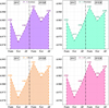 |
Fig. 6 A four-fill area plot for the performance of the models across phases. |
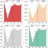 |
Fig. 7 A four-fill fill area plot for the performance of the models across phases. |
Conditioning-based categorization of assessment criteria for the performance of the developed models.
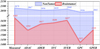 |
Fig. 8 Spline plot to represent the difference among the models. |
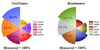 |
Fig. 9 Pie with different radius plots to show the percentage of the model. |
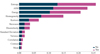 |
Fig. 10 SHAP sensitivity analysis of the best-performed framework. |
4 Conclusion
In the current study, deeper analysis is made of the performance of machine learning models optimized through Escaping Bird Search Optimization: Ada Boost Classifier, Gaussian Process Classifier, and Support Vector Classifier. Such subtleties are attempted to be found through a wide range of measures and visualizations in this study. The approach followed a systematic division of data into discrete subsets for training, testing, and thorough evaluation to gain a sound understanding of model performance that allowed for informed decision-making in clinical diagnosis frameworks. In both the classifications, the SVEB model was performing better concerning the brain tumor and non-tumor classification established with the use of measures like precision, recall, and F1-score at accuracy rates close to 0.990. Indeed, the SVEB model proved to be the most accurate in predicting the cases of brain tumors, accounting for 17.6% of the predictions made in the 100% database. The SVEB model was incredibly able to conduct predictions of up to 2068 and 1657 for brain tumor and nontumor occurrences, respectively, with very small prediction error percentages of 1.5% and 0.5%. The measured values for non-tumor cases were 2079, while for brain tumor cases, they were 1683. All things being equal, the results showcase how much superior the performances of SVEB were in making predictions and also more reliable with increased discriminatory power while classifying brain tumors. The comparative performances by the various models, such as ADAC and ADEB, have shown the need for full awareness of the subtleties in choosing and optimizing a model. Through the provision of insightful information about predictive capacities and their implications for clinical decision-making, this work advances the understanding of machine learning applications in neuro-oncology. Future advancements in the field of brain tumor categorization could lead to better patient outcomes and increased diagnostic precision through the development of prediction algorithms.
Funding
This work was supported by the Natural Science Foundation of China (No. 62102147), in part by the Key Scientific Research Foundation of Hunan Provincial Department of Education (Nos. 23A0575, 24A0598), in part by the Hunan Provincial Natural Science Foundation (Nos. 2024JJ7184, 2024JJ7187), in part by the Guiding Science and Technology Plan Project of Yongzhou City (No. 2024YZ011), in part by the Research Project of Hunan University of Science and Engineering (No. 24XKYZC03), in part by the Teaching Reform Research Project of Hunan University of Science and Engineering (No. XKYJ2024012), in part by the construct program of applied characteristic discipline in Hunan University of Science and Engineering, and in part by the Aid program for Science and Technology Innovative Research Team in Higher Educational Instituions of Hunan Province.
Conflicts of interest
The authors declare no conflicts of interest.
Data availability statement
Data can be shared upon request.
Author contribution statement
TH performed Data collection also XY carried out simulation and analysis. EJ evaluate the first draft of the manuscript, editing and writing.
References
- G. Çınarer, B.G. Emiroğlu, Classification of brain tumors by machine learning algorithms, in 2019 3rd International Symposium on Multidisciplinary Studies and Innovative Technologies (ISMSIT), IEEE (2019) pp. 1–4 [Google Scholar]
- A. Omuro, L.M. DeAngelis, Glioblastoma and other malignant gliomas: a clinical review, JAMA 310, 1842–1850 (2013) [Google Scholar]
- M. Weller et al., Glioma, Nat. Rev. Dis. Primers 1, 1–18 (2015) [Google Scholar]
- M.L. Bondy et al., Brain tumor epidemiology: consensus from the brain tumor epidemiology consortium, Cancer 113, 1953–1968 (2008) [CrossRef] [Google Scholar]
- J. Amin, M. Sharif, M. Raza, M. Yasmin, Detection of brain tumor based on features fusion and machine learning, J. Ambient Intell. Humanized Comput. 15, 1–17 (2024) [Google Scholar]
- D.P.R. Chieffo, F. Lino, D. Ferrarese, D. Belella, G.M. Della Pepa, F. Doglietto, Brain tumor at diagnosis: from cognition and behavior to quality of life, Diagnostics 13, 541 (2023) [CrossRef] [Google Scholar]
- G. Katti, S.A. Ara, A. Shireen, Magnetic resonance imaging (MRI) − a review, Int. J. Dental Clin. 3, 65–70 (2011) [Google Scholar]
- T.M. Buzug, Computed tomography, in Springer handbook of medical technology, Springer (2011) pp. 311–342 [Google Scholar]
- P.Y. Wen et al., Updated response assessment criteria for high-grade gliomas: response assessment in neuro-oncology working group, J. Clin. Oncol. 28, 1963–1972 (2010) [CrossRef] [Google Scholar]
- Y.P. Singh, D.K. Lobiyal, A comparative analysis and classification of cancerous brain tumors detection based on classical machine learning and deep transfer learning models, Multimedia Tools Appl. 83, 39537–39562 (2024) [Google Scholar]
- D.A. Reardon et al., Immunotherapy advances for glioblastoma, Neuro Oncol. 16, 1441–1458 (2014) [CrossRef] [Google Scholar]
- D. Black et al., Towards machine learning-based quantitative hyperspectral image guidance for brain tumor resection, Commun. Med. 4, 131 (2024) [CrossRef] [Google Scholar]
- S.U.R. Khan, M. Zhao, S. Asif, X. Chen, Hybrid‐NET: a fusion of DenseNet169 and advanced machine learning classifiers for enhanced brain tumor diagnosis, Int. J. Imaging Syst. Technol. 34, e22975 (2024) [CrossRef] [Google Scholar]
- M. Celik, O. Inik, Development of hybrid models based on deep learning and optimized machine learning algorithms for brain tumor Multi-Classification, Expert Syst. Appl. 238, 122159 (2024) [CrossRef] [Google Scholar]
- M. Rivera, S. Norman, R. Sehgal, R. Juthani, Updates on surgical management and advances for brain tumors, Curr. Oncol. Rep. 23, 1–9 (2021) [CrossRef] [Google Scholar]
- C. Turnquist, B.T. Harris, C.C. Harris, Radiation-induced brain injury: current concepts and therapeutic strategies targeting neuroinflammation, Neurooncol. Adv. 2, vdaa057 (2020) [Google Scholar]
- J.L. Martínez-Tlahuel et al., Chemotherapy for brain tumors BT, in Principles of Neuro-Oncology: Brain & Skull Base, edited by A. Monroy-Sosa, S.S. Chakravarthi, J.G. de la Garza-Salazar, A. Meneses Garcia, and A.B. Kassam (Springer International Publishing, Cham, 2021), pp. 357–383 [Google Scholar]
- B. Ganjeifar, F.S. Morshed, Targeted drug delivery in brain tumors-nanochemistry applications and advances, Curr. Topics Med. Chem. (2021) http://dx.doi.org/10.2174/1568026620666201113140258. [Google Scholar]
- J. Blakeley, Drug delivery to brain tumors, Curr. Neurol. Neurosci. Rep. 8, 235–241 (2008) [CrossRef] [Google Scholar]
- M. Aryal, T. Porter, Emerging therapeutic strategies for brain tumors, Neuromolecular Med. 24, 23–34 (2022) [CrossRef] [Google Scholar]
- S. Anantharajan, S. Gunasekaran, T. Subramanian, R. Venkatesh, MRI brain tumor detection using deep learning and machine learning approaches, Measurement: Sens. 31, 101026 (2024) [CrossRef] [Google Scholar]
- M.L. Montoya, N. Kasahara, H. Okada, Introduction to immunotherapy for brain tumor patients: challenges and future perspectives, Neurooncol. Pract. 7, 465–476 (2020) [Google Scholar]
- T.J. Kaufmann et al., Consensus recommendations for a standardized brain tumor imaging protocol for clinical trials in brain metastases, Neuro Oncol. 22, 757–772 (2020) [CrossRef] [Google Scholar]
- P. Domingos, A few useful things to know about machine learning, Commun. ACM 55, 78–87 (2012) [CrossRef] [Google Scholar]
- T. Hastie, R. Tibshirani, J.H. Friedman, J.H. Friedman, The Elements of Statistical Learning: Data Mining, Inference, and Prediction 2 (Springer, 2009) [Google Scholar]
- D. Bassir, H. Lodge, H. Chang, J. Majak, G. Chen, Application of artificial intelligence and machine learning for BIM, Int. J. Simulat. Multidiscip. Des. Optim. 14, 5 (2023) [CrossRef] [EDP Sciences] [Google Scholar]
- A. Mosavi, Application of data mining in multiobjective optimization problems, Int. J. Simul. Multidiscip. Des. Optim. 5, A15 (2014) [CrossRef] [EDP Sciences] [Google Scholar]
- Y. Freund, Boosting a weak learning algorithm by majority, Inf. Comput. 121, 256–285 (1995) [CrossRef] [Google Scholar]
- P.S. Efraimidis, P.G. Spirakis, Weighted random sampling with a reservoir, Inf. Process Lett. 97, 181–185 (2006) [CrossRef] [Google Scholar]
- C.E. Rasmussen, C.K.I. Williams, Gaussian Processes for Machine Learning 1 (Springer, 2006) [Google Scholar]
- H. Nickisch, C.E. Rasmussen, Approximations for binary Gaussian process classification, J. Mach. Learn. Res. 9, 2035–2078 (2008) [MathSciNet] [Google Scholar]
- J. Quinonero-Candela, C.E. Rasmussen, A unifying view of sparse approximate Gaussian process regression, J. Mach. Learn. Res. 6, 1939–1959 (2005) [MathSciNet] [Google Scholar]
- T.P. Minka, A family of algorithms for approximate Bayesian inference (Massachusetts Institute of Technology, 2001) [Google Scholar]
- V. Vapnik, Statistical Learning Theory (John Willey & Sons, Inc., New York, 1998) [Google Scholar]
- S. Maldonado, J. Pérez, R. Weber, M. Labbé, Feature selection for support vector machines via mixed integer linear programming, Inf. Sci. (N Y) 279, 163–175 (2014) [CrossRef] [Google Scholar]
- C.-C. Chang, C.-J. Lin, LIBSVM: a library for support vector machines, ACM Trans. Intell. Syst. Technol. 2, 1–27 (2011) [CrossRef] [Google Scholar]
- M. Aydogdu, M. Firat, Estimation of failure rate in water distribution network using fuzzy clustering and LS-SVM methods, Water Resour. Manag. 29, 1575–1590 (2015) [CrossRef] [Google Scholar]
- A. Géron, Hands-on Machine Learning with Scikit-Learn, Keras, and TensorFlow (O'Reilly Media, Inc., 2022) [Google Scholar]
- A. Hedenström, M. Rosén, Predator versus prey: on aerial hunting and escape strategies in birds, Behavior. Ecol. 12, 150–156 (2001) [CrossRef] [Google Scholar]
- D. Lentink et al., How swifts control their glide performance with morphing wings, Nature 446, 1082–1085 (2007) [CrossRef] [Google Scholar]
- H.C. Howland, Optimal strategies for predator avoidance: the relative importance of speed and manoeuvrability, J. Theor. Biol. 47, 333–350 (1974) [CrossRef] [Google Scholar]
- M. Shahrouzi, A. Salehi, Design of large-scale structures by an enhanced metaheuristic utilizing opposition-based learning, in 2020 4th Conference on Swarm Intelligence and Evolutionary Computation (CSIEC), IEEE (2020) pp. 27–31 [Google Scholar]
Cite this article as: Tangsen Huang, Xiangdong Yin, Ensong Jiang, Decision-making in clinical diagnostic for brain tumor detection based on advanced machine learning algorithm, Int. J. Simul. Multidisci. Des. Optim. 16, 1 (2025)
All Tables
Conditioning-based categorization of assessment criteria for the performance of the developed models.
All Figures
|
Fig. 1 The plot illustrates the correlation between the input and output. |
| In the text | |
|
Fig. 2 The histogram-normal distribution plot for inputs and output. |
| In the text | |
|
Fig. 2 (Continued). |
| In the text | |
|
Fig. 3 The flowchart of the ADAC. |
| In the text | |
|
Fig. 4 3D plot for the convergence curve of the three models. |
| In the text | |
|
Fig. 5 A four-fill area plot for the performance of the models across phases. |
| In the text | |
|
Fig. 6 A four-fill area plot for the performance of the models across phases. |
| In the text | |
|
Fig. 7 A four-fill fill area plot for the performance of the models across phases. |
| In the text | |
|
Fig. 8 Spline plot to represent the difference among the models. |
| In the text | |
|
Fig. 9 Pie with different radius plots to show the percentage of the model. |
| In the text | |
|
Fig. 10 SHAP sensitivity analysis of the best-performed framework. |
| In the text | |
Current usage metrics show cumulative count of Article Views (full-text article views including HTML views, PDF and ePub downloads, according to the available data) and Abstracts Views on Vision4Press platform.
Data correspond to usage on the plateform after 2015. The current usage metrics is available 48-96 hours after online publication and is updated daily on week days.
Initial download of the metrics may take a while.