


| Issue |
Int. J. Simul. Multidisci. Des. Optim.
Volume 17, 2026
|
|
|---|---|---|
| Article Number | 16 | |
| Number of page(s) | 19 | |
| DOI | https://doi.org/10.1051/smdo/2026012 | |
| Published online | 31 July 2026 | |
Research article
Optimization and early warning strategy for wind turbine blade acoustic signature monitoring array based on wind farm simulation
1
State Energy Tengxian Energy Development Co., Ltd., Nanning 530004, PR China
2
College of Electrical Engineering, Guangxi University, Nanning 530004, PR China
* e-mail: This email address is being protected from spambots. You need JavaScript enabled to view it.
Received:
19
April
2026
Accepted:
2
June
2026
Abstract
Complex wind farm environments cause severe spatial aliasing and signal attenuation in blade acoustic signature monitoring. This paper presents an acoustic sensor array topology optimization method based on multi-physics simulation for high-fidelity acquisition of weak voiceprint features. A three-dimensional sound field model coupling aerodynamic noise and mechanical vibration quantifies sound propagation under varying wind speeds and yaw angles. A heuristic particle swarm algorithm discretely optimizes microphone array coordinates on tower and nacelle surfaces by maximizing the signal-to-noise ratio. A surrogate model accelerates sound field evaluation while eliminating nodes disturbed by strong wind vortices. Experiments on a public blade crack acoustic dataset show that the optimized array reduces normalized root mean square error by 44.4 percent compared to conventional spiral arrays, and the proposed attention-based multi-scale network achieves an area under the curve of 0.967 and recall of 0.913.
Key words: Wind turbine blade / acoustic signature monitoring / acoustic array optimization / multi-physics simulation / deep learning
© B. Zou and J. Liu, Published by EDP Sciences, 2026
 This is an Open Access article distributed under the terms of the Creative Commons Attribution License (https://creativecommons.org/licenses/by/4.0), which permits unrestricted use, distribution, and reproduction in any medium, provided the original work is properly cited.
1 Introduction
As one of the renewable and clean energy sources with the most potential for large-scale development, wind energy plays an increasingly key role in the transformation of global energy structure. By 2025, the cumulative installed capacity of global wind power has exceeded 1.2 Terawatts (TW), among which the proportion of offshore wind power and large blade units in the low wind speed zone of onshore continues to rise [1]. As the core aerodynamic component of wind turbine to capture wind energy, the blade is exposed to multiple stress coupling effects such as alternating aerodynamic load, centrifugal force, sand erosion and lightning strike for a long time. Its structural health state directly determines the safe operation and whole life cycle economy of the unit. According to statistics, unplanned downtime caused by blade failure accounts for more than 20% of the total downtime of wind turbines, and the maintenance cost of a major blade failure accident can be as high as 15% to 20% of the individual cost [2]. Therefore, the development of blade condition monitoring and early warning technology with high reliability, low cost and online deployment has become a common key problem to be broken through in the field of wind power operation and maintenance. Similar multi-source fusion strategies have been explored in other domains, providing methodological reference for acoustic sensor networks [3]. The idea of multi-source data fusion can provide reference for information fusion of multi-sensor acoustic monitoring systems in wind farms.
Among the existing methods for structural health monitoring, the acoustic signature monitoring technology based on acoustic signals has attracted much attention due to its advantages of non-contact, high sensitivity, and rapid response to early micro-crack propagation. A microphone array is installed on the surface of the tower or nacelle to collect the aerodynamic noise and mechanical vibration sound waves radiated during blade sweeping. Subsequently, the weak voice pattern characteristics representing structural damage are extracted to realize the early identification of typical faults such as cracks, delamination, and edge erosion. However, the harsh acoustic environment of complex wind farms makes this technology face severe challenges in practical application. On the one hand, the blades are operating in the interference between unsteady incoming flow and tower wake, and the radiated sound waves experience significant shear layer refraction, atmospheric turbulence scattering and tower diffraction effects on the propagation path, resulting in serious spatial aliasing and amplitude attenuation of the acoustic signals arriving at the sensor [4]. On the other hand, the mechanical noise of the engine room itself, the high-frequency component of gearbox meshing and the friction noise of yaw system constitute high-intensity background interference, which makes the weak voice-pattern characteristics that represent the early damage of the blade easily submerged. The coupling effect of the above factors leads to the sharp degradation of the beamforming performance of the traditional fixed geometry array under complex operating conditions, such as the main lobe widening and side lobe elevation, and the spatial resolution and Signal-to-Noise Ratio (SNR) of sound source localization are far lower than those expected by the ideal free field design [5].
For the design of acoustic monitoring arrays for wind turbine blades, there are three main technical paths. The first path relies on the classical array signal processing theory, adopts regular geometric configurations such as uniform linear array, cross array or Archimedean spiral array, and uses beamforming or deconvolution methods to image sound sources. This kind of method is simple to implement and has good robustness. However, its design is completely based on the assumption of free field and far-field plane wave, and the distortion effect of the actual flow in the wind field on the acoustic propagation path is not taken into consideration, which leads to the performance deviation from the design index after field deployment [6]. The second path introduces numerical optimization algorithms to sparsity design the array topology, represented by genetic algorithms, simulated annealing, or Particle Swarm Optimization (PSO), to automatically search for sensor locations by maximizing the number of array manifold conditions or minimizing side-lobe levels. Such methods improve the adaptive ability of the array to specific sound source distribution to a certain extent, but the sound field evaluation in the optimization process still relies on the simplified point source propagation model, which fails to effectively couple the physical generation mechanism of fan aerodynamic noise with the propagation and attenuation law under complex boundaries [7]. The third approach attempts to use computational aeroacoustics or finite element methods to conduct high-fidelity numerical simulations of the blade sound field to guide sensor placement. Although this method has significant advantages in the accuracy of acoustic propagation modeling, the huge time required for a single solution of high-fidelity simulation makes it unaffordable to directly insert it into the iterative optimization loop. It is usually only used for post hoc verification of a few preset schemes, rather than to drive the active optimization of array configurations [8].
In summary, although the existing studies have made beneficial progress in their respective dimensions, there are still significant deficiencies in three levels. Firstly, at the level of sound field modeling, there is no surrogate model for sound propagation that can not only accurately describe the refraction of shear layer and the scattering effect of tower, but also respond quickly in the optimization iteration. As a result, it is difficult to balance the physical reality and computational feasibility of the array design. Secondly, at the array optimization level, the existing heuristic search strategies do not make full use of the high-dimensional physical information provided by the sound field simulation to guide the search direction, resulting in low optimization efficiency and easy to fall into the local optimum. Thirdly, at the system integration level, the array layout design and the subsequent voiceprint early warning algorithm are in a state of separation for a long time – the former pursues the single optimum of acoustic imaging quality, and the latter relies on the quality of voiceprint features extracted from the acquired signal. There is a lack of closed-loop feedback based collaborative design mechanism between the two. The above limitations constitute the immediate entry point of this study.
In order to systematically solve the above problems, this paper proposes a design and warning framework for fan blade voice-pattern monitoring array by integrating multi-physics simulation, surrogate model acceleration and closed-loop feedback optimization. The framework takes the optimization of acoustic sensor array topology as the core, and takes the high-fidelity acquisition and reliable identification of early crack voiceprint features as the ultimate goal. Aerodynamic noise generation, complex boundary sound propagation, array signal processing and the warning model is integrated into a unified collaborative optimization system. Specifically, firstly, a three-dimensional sound field simulation model of the coupling of aerodynamic noise and mechanical vibration of the blade was established, and the sound propagation path and attenuation law under different wind speed, yaw Angle and blade tip speed ratio were systematically quantified. Secondly, an array optimization model was constructed to maximize the SNR of the monitoring area, and Kriging surrogate model was introduced to approximately accelerate the high-cost sound field simulation. On this basis, a discrete topology search algorithm coupled with the surrogate model and the heuristic PSO mechanism was designed. Under the premise of meeting the sensor spacing constraints and hardware cost constraints, the redundant sensor nodes disturbed by strong wind noise and eddy current were dynamically eliminated, and the optimal array spatial configuration was output. Finally, the beamforming pattern collected by the optimized array was fed into the attention mechanism based multi-scale voice recognition network, and the sensitivity gradient of the warning network to the input SNR was used to reverse guide the further fine-tuning of the array layout, forming a self-consistent closed loop from “optimal acquisition” to “reliable warning”.
Based on the above research ideas, this paper has completed the following main work and achieved corresponding results. At the theoretical modeling level, a 3D wind farm sound propagation simulation model coupled with the Amiet trailing edge noise model and ray-tracing shear layer correction was constructed, and a sound field database covering typical operating conditions was generated by parametric scanning. At the level of algorithm design, a PSO algorithm assisted by surrogate model is proposed, which achieves a significant reduction in the computational cost of sound field simulation and a significant improvement in the search efficiency. At the system validation level, the beamforming performance of the optimized array and the accuracy of subsequent crack warning were comprehensively evaluated and compared based on the public data set of acoustic detection of trailing edge cracks of Delft University of Technology (TU Delft) wind turbine blades.
The main innovations and contributions of this work include:
The Cooperative PSO - Surrogate Model (CPSO-SM) algorithm is proposed, which is an acoustic array topology optimization algorithm coupling the heuristic PSO mechanism and Kriging surrogate model. Unlike existing sparse optimization methods that rely on free-field assumptions or isolated post-hoc acoustic corrections, CPSO-SM uniquely integrates shear-layer refraction and tower scattering physical constraints directly into the iterative loop. By dynamically updating the Kriging surrogate model's accuracy during optimization and introducing the eddy current interference penalty function, the algorithm significantly improves the search efficiency and solution quality of the optimal array configuration under complex acoustic field constraints.
A dual-attention-driven multi-scale voiceprint feature extraction network was designed to enhance the ability to represent the crack-induced weak voiceprint components through the joint attention weighting of the channel dimension and the time dimension.
A closed-loop iterative strategy from acoustic field simulation to array optimization and then to early warning evaluation is established to realize the end-to-end collaborative optimization of array layout parameters and early warning network input quality.
The rest of this paper is organized as follows: Section 2 systematically reviews the relevant literature in the field of wind turbine blade acoustic monitoring, array layout optimization, and multi-physics simulation, and clearly points out the existing research gaps. Section 3 elaborates the proposed methodology, including the multi-physics coupled sound field simulation model, the CPSO-SM array optimization algorithm, and the mathematical description and implementation details of the AMAF-Net voiceprint early warning network. Section 4 describes the experimental design and evaluation protocol, including data sets, baseline methods, evaluation metrics, and implementation parameters. In Section 5, the array optimization results, crack warning performance, and ablation analysis are reported, supplemented by a typical case analysis. In Section 6, the experimental results are discussed, and the applicable boundaries and limitations of the method are analyzed. Section 7 summarizes the work in this paper and looks forward to future research directions.
2 Literature review
2.1 Modeling of aerodynamic noise mechanism and propagation in blades
The physical basis of sound pattern monitoring of fan blades lies in the accurate recognition of the sound field radiated by the blades and its propagation law. Blade noise is mainly dominated by trailing edge noise generated by the interaction between turbulent boundary layer and trailing edge, followed by tip vortex shedding noise and laminar separation noise [9]. For noise source modeling, the Amiet trailing edge noise theory has been widely adopted due to its good balance between prediction accuracy and computational efficiency. The theory relates the unsteady pressure spectrum of airfoil surface to the far-field sound pressure spectrum through the transfer function [10]. However, the Amiet model is based on the assumption of uniform incoming flow and infinite wingspan, which makes it difficult to accurately describe the modulation effect of three-dimensional blade rotation and incoming flow turbulence. At the sound propagation level, the process of sound wave radiation from the blades to the tower or engine sensors in the actual wind power plant is affected by multiple physical mechanisms: the vertical wind shear and temperature gradient of the atmospheric boundary layer cause the sound ray bending and the formation of the sound shadow region [4]. As a large blunt-body structure, the tower generates diffraction and reflection. The periodic Doppler shift caused by blade rotation renders the received signal spectrum nonstationary. Some studies use computational aeroacoustics methods to couple large eddy simulation and acoustic ratio equations to achieve high-fidelity integrated solution of near-field sound source and far-field propagation of blades [8]. Although this kind of method has high physical completeness, it is difficult to support the array optimization task that requires a large number of iterations when tens of thousands of cores are needed to solve a single working case [11].
2.2 Microphone array signal processing and sound source imaging
Microphone array is the front-end acquisition hardware of acoustic signature monitoring, and its signal processing algorithm performance directly determines the quality of subsequent voiceprint feature extraction. Beamforming is the most mature sound source imaging technique in this field. It compensates the propagation delay of the received signal of each array element and forms a spatially selective gain by alignment and summation. The spatial resolution of conventional delayed summation beamforming is limited by the Rayleigh criteria, where the main lobe width is inversely proportional to the array aperture [6]. In order to break through this limitation, the deconvolution method represented by CLEAN based on Spatial Correlation (CLEAN-SC) significantly improves the spatial resolution and dynamic range by iteratively removing the side lobe components in the point spread function [12]. In recent years, the theory of compressed sensing has been introduced into the field of sound source imaging, and the sparse prior of sound source space is used to achieve high-resolution identification under the condition that the number of array elements is much smaller than Nyquist's requirement [13]. Although the above algorithms perform well under ideal free-field conditions, they generally face performance degradation when deployed in wind farms. The fundamental reason is that the spherical wavefront assumed by beamforming is distorted after experiencing the refraction of the shear layer, resulting in the mismatch between the theoretical delay and the actual arrival delay, which leads to the main lobe directional deviation and the decline of focusing ability. Although ray tracing-based delay correction methods have been proposed, such methods require the shear layer velocity profile to be known, and the real-time and accurate measurement of the field wind velocity profile is itself a challenge [14].
2.3 Optimal design of sensor array layout
The spatial configuration of the array is another key factor in determining the performance of sound source imaging. Regular geometric array has been dominant for a long time because of its simple design and calibration, but its beam pattern is uniquely determined by the geometric configuration, which lacks the adaptability to the specific sound field environment. The core of sparse array optimization method is to optimize the maximum sidelobes level of beampattern or the condition number of array manifold by optimizing the sensor position under the constraint of the total number of array elements. The solution method includes heuristic strategies such as genetic algorithm, PSO and differential evolution [15]. It is worth noting that most of the existing array optimization studies are based on the assumption of free-field propagation, and the transfer function from the sound source to the sensor is reduced to a spherical wave model only dependent on distance. This simplification makes it difficult for the optimized configuration to cope with the propagation path distortion caused by shear layer refraction, tower scattering and atmospheric turbulence in the wind farm. A few studies have attempted to embed a two-dimensional parabolic equation propagation model in the optimization, but the computational overhead is still high, and the coupling effect of blade rotation and tower 3D diffraction cannot be accurately captured. How to balance the physical fidelity and computational feasibility of propagation modeling in the array optimization cycle is a bottleneck problem that has not been effectively solved at present.
2.4 DL-driven voiceprint feature extraction
With the successful application of DL in speech recognition and environmental acoustics, data-driven voiceprint feature learning methods have been introduced into the field of wind turbine blade damage identification [16]. Convolutional neural networks have been widely used in acoustic spectrum classification due to their ability to capture time-frequency local patterns. The introduction of attention mechanism further improves the ability of models to focus on weak variciform components [17,18]. In terms of DL anomaly detection, Zhong proposed Deep Internet of Things–Hybrid Anomaly Detection (DeepIoT-HAD), an IoT anomaly detection method based on Deep Autoencoder and hierarchical architecture, which effectively processed high-dimensional data and reduced computing resource consumption through hierarchical architecture [19]. The hierarchical feature extraction strategy can provide a technical reference for the hierarchical characterization of the voice pattern characteristics of fan blades. Although Deep Learning (DL) methods have achieved encouraging recognition accuracy under controlled conditions, their generalization ability in real wind farms still faces severe tests. The first obstacle is the extreme lack of labeled data: the cost of obtaining acoustic samples for blade damage conditions is high, and the size of the training set and the diversity of damage patterns are far from being enough to support the full training of the deep network. Secondly, the voiceprint feature drift caused by the change of operating conditions causes the performance of the model to decay sharply, and it is not practical to collect full coverage data for all operating conditions. In addition, the existing models generally lack correlation with the physical generation mechanism of blade noise, and the decision-making process is difficult to be explained from the acoustic principle, which limits the degree of trust in the actual operation and maintenance [20].
2.5 Comparative analysis of existing methods
In order to clearly present the similarities and differences of the above various methods, Table 1 systematically compares the representative methods from the four dimensions of theoretical basis, acoustic field modeling accuracy, array optimization ability and computational cost.
Comparison of acoustic monitoring array design methods for fan blades.
2.6 Identified research gaps
Based on the above systematic sorting and comparative analysis, there are three clear gaps in the current research, which constitute the direct entry points of this work.
First, there is a lack of array topology design methods that couple physical simulation with efficient optimization. The existing regular array is difficult to adapt to the complex sound field environment. The sparse optimization of free field does not take into account the propagation distortion effect, and the high-fidelity simulation cannot be embedded in iterative optimization due to the high computational cost. There is an urgent need to develop an array optimization framework that can not only accurately characterize the key physical mechanisms such as shear layer refraction and tower scattering, but also enable rapid sound field evaluation through surrogate models.
Second, there is no targeted feature enhancement mechanism for weak crack voiceprint. The existing DL methods have inherent defects in the lack of labeled data and the generalization of working conditions, and the network architecture design does not fully consider the weakness and frequency domain sparsity of crack-induced voiceprint, which makes the detection rate of early damage difficult to meet the needs of preventive operation and maintenance. Third, there is a lack of closed-loop feedback synergy between the array layout and the warning algorithm. The current array design and the subsequent damage identification algorithm are in an isolated serial state. The former aims at acoustic imaging quality while the latter aims at classification accuracy. How to realize the end-to-end joint optimization of array parameters and early warning model parameters under a unified framework is the key to improve the comprehensive efficiency of the monitoring system.
3 Methodology
3.1 Overall framework
The framework proposed in this paper is composed of three core modules: multi-physics coupled sound field simulation and propagation modeling module, surrogate model-assisted particle swarm array topology optimization module (CPSO-SM), and attention mechanism based multi-scale voiceprint feature extraction and warning module (Attention Mechanism based Multi-scale Audio Feature Network, AMAF-Net). The three modules do not operate in isolation, but form a self-consistent collaborative optimization system through closed-loop joint training strategy. Figure 1 shows the overall architecture and data flow diagram of the framework.
The framework operation process can be summarized as the following stages. Firstly, the 3D sound field simulation model of the blade was established based on the computational aeroacoustics and ray tracing method, and the sound propagation database covering typical operating conditions was generated by parametric scanning. Secondly, the Kriging surrogate model is trained using the database to replace the high-cost simulation, and the surrogate model is embedded in the discrete PSO algorithm to search for the array topology that maximizes the SNR of the monitoring area under the constraint of the number and spacing of sensors. Thirdly, based on the beamforming time-frequency feature map collected by the optimized array, the AMAF-Net is sent to extract the voice pattern features of cracks and identify the damage state. Finally, the gradient of the early-warning network loss function with respect to the array coordinates is calculated, which is used as a feedback signal to guide the further fine-tuning of the array layout to achieve end-to-end closed-loop optimization from “optimal acquisition” to “reliable early-warning”. Table 2 shows the key notations used in this article.
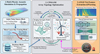 |
Fig. 1 Overall architecture and data flow of the proposed CPSO-SM and AMAF-Net joint optimization framework. |
Description of key symbols.
3.2 Simulation and propagation modeling of multi-physics coupled blade sound field
It is a physical prerequisite for array topology optimization to accurately describe the propagation law of acoustic waves radiated by blades in complex wind field environment. This section discusses aerodynamic noise source modeling, propagation path modification and parametric simulation database construction at three levels.
3.2.1 Modeling of aerodynamic noise sources
The aerodynamic noise of fan blades is mainly composed of the trailing edge noise of turbulent boundary layer. In this paper, the sound source model of the blade surface is constructed by the Amiet trailing edge noise theory, which relates the unsteady pressure fluctuation spectrum of the airfoil surface to the far-field sound pressure spectrum by the transfer function. For a blade section with an incoming flow velocity of U∞ and an airfoil chord length of c, the far-field sound pressure power spectral density of the trailing edge noise can be expressed as:
 (1)
(1)
where Φpp(ω) is the unsteady pressure spectrum of the airfoil surface, L is the spanwise correlation length, re is the effective acoustic propagation distance, Uc is the convective velocity, and  is the transfer function considering airfoil geometry and incoming flow Angle of attack. The pressure spectrum
  is parametrized using the Goody model, which has good prediction accuracy for both attached and separated boundary layers in the moderate Reynolds number range.
The sound source distribution on the blade surface showed significant heterogeneity along spanwise and chord directions. To this end, the blade is discretized into several spanwise strips, and the chordwise source distribution in each strip is determined by the local airfoil, relative velocity and Angle of attack. The relative velocity Wj of the JTH strip is obtained by synthesizing the rotational velocity with the incoming flow velocity vector:
 (2)
(2)
where Ω is the rotational angular velocity of the wind wheel, and rj is the radius of the strip's spanwise position. The local Angle of attack corresponding to the strip should be solved iteratively by the blade element momentum theory, considering the 3D rotational ascending effect and inflow distortion caused by tower obstruction.
3.2.2 Shear layer refraction and column scattering effect correction
Sound waves radiated from the blade surface need to penetrate the shear layer downstream of the wind wheel in the process of propagation to the tower or engine room sensor. The velocity and temperature differences on both sides of the shear layer led to the refraction of the sound ray, which makes the actual propagation path of the sound wave deviate from the straight line. If the assumption of straight-line propagation in uniform medium is still adopted, the error of time delay estimation and the deviation of amplitude attenuation will not be neglected.
In this paper, the ray tracing method is used to correct the shear layer refraction effect. Considering the two-dimensional shear layer profile U(z), the acoustic ray trajectory satisfies the generalized form of Snell's law:
 (3)
(3)
where θ(z) is the Angle between the ray and the horizontal direction, and c(z) is the local speed of sound. The actual path length Lray and the propagation delay τray of the acoustic wave from the source point xs to the sensor  can be obtained by numerical integration of the differential equation. The corresponding frequency domain transfer function is modified as:
 (4)
(4)
where  for the free field green's function,
  for refraction introduce additional time delay, Ascat is the amplitude correction factor caused by the scattering of the tower.
The modeling of the scattering effect of the tower is based on the theory of cylindrical diffraction. For a tower cylinder with diameter Dt, the scattered sound field caused by acoustic incident can be expressed as the superposition of the cylindrical wave modes of each order. In the frequency range of interest in this paper (500 Hz to 5 kHz), the condition of  is approximately satisfied, and the asymptotic solution of geometric diffraction theory can be used to approximate the scattered field, which greatly reduces the computational complexity. The correction factor Ascat is expressed as:
 (5)
(5)
where Rn is the complex reflection coefficient of the n diffracted ray, and ΔLn is the path difference of the ray with respect to the direct path.
The above shear layer refraction correction together with the tower scattering correction constitutes a complete physical description of the acoustic propagation path. In order to visually present the sound propagation correction process from the blade sound source to the tower/engine room sensor, Figure 2 presents the overall architecture of the multi-physics coupled sound propagation modeling. As shown in the figure, the process successively covers the four stages of blade aerodynamic noise source modeling, shear layer ray tracing correction, tower diffraction and scattering compensation, and the final transfer function synthesis. The output of each stage is transferred step by step. The resulting embeddable array optimization loop correction transfer function  .
.
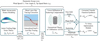 |
Fig. 2 Architecture of multi-physics acoustic propagation modeling. |
3.2.3 Construction of parametric sound field simulation database
In order to support the sound field evaluation requirements of a large number of candidate configurations for subsequent array optimization, it is necessary to construct a parametric sound field simulation database covering typical operating conditions. Wind speed U∞, yaw Angle θy and tip speed ratio λTSR were selected as three independent operating conditions parameters, and discrete sampling was performed in the typical value range of each parameter. The wind speed covers the cut wind speed to rated wind speed interval [4,12]m/s, the yaw Angle covers  , and the tip speed ratio covers [6,9]. The three-parameter orthogonal combination generated a total of
  simulation cases.
The pressure distribution and near-field flow parameters on the blade surface were obtained by solving the Reynolds average Navier-Stokes flow field, and the sound source distribution on the blade surface was calculated based on the Amiet model. Finally, the ray tracing method was used to calculate the corrected transfer function from each preset grid point to the candidate sensor positions in the tower and engine room. All sound field data were stored in the form of frequency domain complex sound pressure matrix, and a fast-indexing mechanism was established to facilitate subsequent surrogate model training and array evaluation calls.
3.3 Surrogate model-assisted heuristic array topology optimization
Based on the acquisition of the parametric sound field database, this section elaborates the design details of the discrete particle swarm array topology optimization algorithm CPSO-SM based on the surrogate model acceleration.
3.3.1 Array performance evaluation function
The goal of array topology optimization is to find the set of sensor space coordinates A that maximizes the average SNR in the monitored region, given the constraints of the number of sensors Nm and the minimum spacing dmin. The monitoring region Ωmon is defined as the 3D space region in front of the blade sweep plane covering the typical damage-prone location.
For A candidate array configuration A, its beamforming output power under a certain condition can be expressed as follows:
 (6)
(6)
where  is the cross-spectral density matrix element of the i and j sensor received signals,
  is the propagation delay from the focus x to the i sensor, This delay is calculated using the modified transfer function of equation (4). The SNR in the monitoring area was defined as the ratio of the beam output power when focusing on the location of the damaged sound source to the average power in the background noise area:
 (7)
(7)
where ωc is the central angular frequency of the characteristic frequency band of the crack voiceprint, and Ωbg is the background region without sound source. Integrating the SNR of several representative operating conditions, the array performance evaluation function is defined as:
 (8)
(8)
where Nc is the number of selected representative working conditions, wc is the probability weight of each working condition, the second term is the penalty term, which is used to suppress the large fluctuation of SNR between different working conditions, and γ is the penalty coefficient. This objective function takes into account both average performance and robustness.
Constraint conditions including the total number of sensors constraints  (including
  for whether the candidate locations selected indicator variables), And minimum distance constraints
  (for all i ≠ j). The latter is used to prevent spatial sampling redundancy and ill-conditioned cross-spectral matrix caused by small sensor spacing. In the context of this acoustic array topology optimization, equation (8) serves as the equivalent of a compliance function commonly used in structural topology optimization. Rather than minimizing structural compliance, the goal here is to maximize the robust acoustic acquisition capability (SNR) across varying operational conditions while penalizing nodes affected by severe background noise.
3.3.2 Kriging surrogate model aided rapid assessment of sound fields
Direct evaluation of the objective function requires beamforming calculation, and the core of which is to obtain the cross-spectral matrix  of each sensor pair. If the cross-spectral matrix is re-computed from the original sound field database for each candidate array evaluation, the computational overhead is still not negligible, especially when the particle swarm size is large. For this purpose, the Kriging surrogate model is introduced to approximate the objective function J(A).
The Kriging model models the unknown function J(A) as the sum of the global trend term and the local deviation term:
 (9)
(9)
where f(A) is the vector of known basis functions (constant basis is taken in this paper), β is the vector of regression coefficients, and Z(A) is a zero-mean Gaussian process whose covariance function is taken to be of Gaussian type:
 (10)
(10)
where  is the process variance and θl is the hyperparameter of the L dimensional input. Given the training sample set
  , and the model for any new input A* prediction is normal distribution, Its forecast
  and forecasting variance
  is given analytically.
In order to improve the adaptability of the surrogate model in the optimization process, a dynamic sample filling strategy based on the expected improvement criterion was adopted. At the end of each round of PSO optimization, the candidate points with the largest prediction variance and better prediction mean were selected for real objective function evaluation, and added to the training set to update the Kriging model. This strategy effectively balances the global improvement and local optimization requirements of the surrogate model accuracy within a finite simulation budget B.
Figure 3 shows the interactive flow architecture of the surrogate model and PSO search in the CPSO-SM algorithm. As shown in the figure, the optimization process alternates between the surrogate model space and the real physical space: the particle swarm rapidly explores the candidate array configurations under the guidance of the surrogate model, while the surrogate model dynamically updates its accuracy according to the elite samples returned by the particle swarm, and the two form an efficient collaboration.
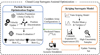 |
Fig. 3 CPSO-SM collaborative architecture. |
3.3.3 Improved discrete particle swarm topology search algorithm
The array topology optimization problem belongs to the category of combinatorial optimization, and the candidate sensor positions are discretized on the preset grid points on the surface of the tower and the cabin cover. In this paper, the standard PSO algorithm is discretized, and dynamic inertia weight and vortex penalty function are introduced to enhance the search performance.
Each particle represents an array configuration, and each dimensional component of the position vector  takes the candidate position index. The particle velocity Vi is defined as the logit value of the position change probability. The location update rule is:
 (11)
(11)
 (12)
(12)
where w is the inertia weight, c1 and c2 are the cognitive and social acceleration coefficients, and  is a random number,
  and
and  are the d dimensional components of the individual historical and global optimal locations, respectively.
  represents the neighborhood set of candidate locations.
  is the sigmoid function.
The inertia weight w is linearly decreasing with the number of iterations:
 (13)
(13)
where  ,
,  to encourage exploration in the early stage and accelerate convergence in the late stage.
In order to avoid the interference region of strong wind noise and eddy current, a penalty function based on the simulation results of flow field is introduced. The eddy current disturbance intensity index  at the candidate position xcand is defined as a function of the average turbulent kinetic energy and the distance from the wall near the position. Particle fitness is modified to
 (14)
(14)
where ηvor is the penalty coefficient. The modified fitness function drives the optimization algorithm to automatically avoids the high turbulence region and selects the position where the flow field is relatively stable to locate the sensor, so as to suppress the background noise interference from the source.
3.4 Multi-scale attention voiceprint feature extraction and early warning
The time-frequency feature map  (T is the number of time frames, F is the number of frequency points) acquired by the optimized array and processed by beamforming contains rich information of blade voice [21]. This section elaborates the AMAF-Net network architecture, aiming to extract discriminative voiceprint representations that are sensitive to crack damage from this feature map.
3.4.1 Dual-attention multi-scale feature extraction network architecture
AMAF-Net adopts the architecture of 1D convolutional backbone network and dual attention mechanism cascade. The backbone network is stacked with four residual convolutional blocks, each containing two expanded convolutional layers, batch normalization, and ReLU activation. The expansion rate was set sequentially to  exponentially expand the receptive field while maintaining the number of parameters, capturing the evolving pattern of crack voiceprint at different time scales. The output feature graph of the backbone network is denoted as
  , where C is the number of channels.
In order to enhance the attention to the crack sensitive frequency band, the squeeze-excitation attention mechanism is introduced in the channel dimension. The channel description vector  is first obtained by global average pooling along the time axis
 (15)
(15)
The channel weight vector  is subsequently generated through the two-layer fully connected network
 (16)
(16)
where δ is ReLU activation, σ is sigmoid activation,  and
and  are the learnable weights, and r is the dimensionality reduction ratio. Weighted after the characteristics of the graph is
  .
.
Furthermore, a self-attention mechanism is introduced in the temporal dimension to capture the long-range dependence of voiceprint events. The query, key, and value matrices are computed for the channel-weighted feature sequence  :
:
 (17)
(17)
where  for projection matrix. The attention weight matrix
  and the output O are
 (18)
(18)
After normalization by the residual connection and layer, the output sequence was flattened and mapped to the binary output (normal/cracked) through the fully connected layer. The overall network structure is shown in Figure 4.
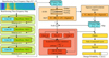 |
Fig. 4 AMAF-Net architecture. |
3.4.2 A contrast learning enhancement strategy for weak voice patterns
In the early stage of crack, the change of voiceprint features is extremely weak, and it is difficult to drive the network to learn enough inter-class separability only by the cross-entropy classification loss. To this end, supervised contrast learning was introduced as an auxiliary training task. Positive sample pairs (from different time periods of the same damage state) and negative sample pairs (from different damage states) were constructed within batches. Let zi be the feature vector output by the AMAF-Net encoder, and the contrast loss is defined as
 (19)
(19)
where  is the index set of positive samples in the same category as sample i, and
  is all samples in the batch except i,
  for the cosine similarity,
  is the temperature coefficient. The contrast loss explicitly Narrows the features of the same type of samples and pushes away the features of different types of samples, which effectively increases the separation between normal and crack cases in feature space.
3.4.3 Warning thresholds are set
The warning threshold τw was determined based on the statistical distribution of the feature vectors of the validation set. For all normal case samples in the validation set, the encoded eigenvector  was calculated, and the mean μ and covariance matrix Σ of the multivariate Gaussian distribution were estimated. For any new sample feature z, calculate the Mahala Nobis distance
 (20)
(20)
The threshold τ was set to the quantile of 95% the Mahalanobis distance of normal samples in the validation set to ensure that the false alarm rate did not exceed 5% under normal operating conditions. In the online monitoring phase, an early warning is triggered when the Mahala Nobis distance of K consecutive time Windows exceeds τ.
3.5 Closed-loop simulation-early warning joint optimization strategy
Although the above array optimization and voiceprint warning module are serial in the initial design, there is potential synergy space between them. This section describes the closed-loop joint training strategy, which feeds the sensitivity of the early warning network to the input quality to the array layout to achieve end-to-end collaborative optimization.
3.5.1 Feedback gradient construction
Set up early warning network output for damage probability  , where F(A) represents the beamforming time-frequency feature map generated by the dependent array configuration A. In the joint training phase, fixed network parameters θAMAF, Calculating early-warning loss
  coordinates relative to the array of
  gradient. Since the feature map generation process involves nondifferentiable beamforming and cross-spectrum matrix calculation, the finite difference method combined with the surrogate model is used to approximate the gradient:
 (21)
(21)
where δ is the small displacement, and ek is the unit vector along the coordinate axis. To reduce the computational overhead, gradients are computed only for some candidate sensors near the global optimal particle.
3.5.2 Joint training process
The joint training total loss function is:
 (22)
(22)
where  encourages the array to move in the direction of improving the warning performance, λ1 and λ2 are equilibrium coefficients. The joint training algorithm 1 is detailed in Appendix A.
4 Experimental design
4.1 Datasets
The acoustic detection data set of fan blade trailing edge cracks published by Delft University of Technology was used in this study [2]. The data set is derived from the aerodynamic noise measurement experiment of the NACA 64-618 airfoil section in a wind tunnel with low turbulence, and includes the acoustic measurement data under four crack lengths of 0 mm, 10 mm, 20 mm and 30 mm. A 64-channel planar microphone array with sampling frequency of 51.2 kHz was used to collect data, which covered the main energy frequency band of blade aerodynamic noise. For each crack condition, the cross-spectrum matrix after fast Fourier transform processing and the corresponding beamforming sound source localization map were provided in the dataset. The map size was 51×51 pixels, corresponding to a 0.8 m×0.8 m sound source scanning plane. In the data preprocessing stage, the beamforming map was divided into normal (0 mm) and crack (10 mm, 20 mm, and 30 mm) labels according to the crack length, and the pixel values of the map were normalized by Z-score to eliminate the dimensional differences. At the same time, the self-spectrum and cross-spectrum information of each microphone channel are extracted from the cross-spectrum matrix, and the array manifold vector is constructed for the input of the array optimization module. The dataset was stratified into a training set (70%), a validation set (15%), and a test set (15%) according to the blade running Angle of attack to ensure that each subset contained a balanced distribution of operating conditions.
4.2 Baseline methods
In order to comprehensively evaluate the performance of the proposed methods, five representative baseline methods were selected for comparison. The first type is the traditional regular array layout, which adopts two configurations, the Archimedean spiral array and the uniform cross array, which are widely used in wind tunnel acoustic measurement [6]. The second type is the free-field sparse optimization array, which adopts the sparse constrained deconvolution array design method based on orthogonal matching pursuit proposed by He et al., which optimates the array element position with the goal of minimizing cross-correlation [13]. The third category is the high-fidelity simulation driven layout, which uses the manual placement scheme of computational aeroacoustic simulation combined with expert experience described in Brandetti et al. as the reference benchmark with the highest simulation accuracy but the most expensive [8]. The fourth type is the traditional voiceprint recognition method, which uses the Mel-Frequency Cepstral Coefficients–Support Vector Machine (MFCC-SVM) classifier and the Wavelet Packet Energy–Random Forest (WPE-RF) classifier. Both are classical shallow models in the field of rotating machinery acoustic fault diagnosis [16]. The fifth category is the DL method, which adopts the ResNet-18 architecture recommended by Gangsar and uses the beamforming map as the input for end-to-end classification [17].
4.3 Evaluation metrics
The evaluation index covers two dimensions of array sound field reconstruction performance and crack warning performance. The Mainlobe Width (at-3 dB, MW) was used to measure the spatial resolution of sound source localization, and the Peak Sidelobe Level (PSL) was used to evaluate the ability of the array to suppress spurious sound sources. The Normalized Root Mean Square Error (NRMSE) was used to quantify the global deviation between the reconstructed sound field and the reference sound field. Five indicators including Accuracy, Precision, Recall, F1-Score and Area Under the Curve (AUC) were used to comprehensively evaluate the performance of crack warning. Accuracy reflects the overall classification accuracy, precision and recall focus on the control ability of false positive rate and false negative rate, respectively. F1 score is the harmonic average of the two, and AUC is the comprehensive discrimination ability of the model under different thresholds. For all indicators, the mean and standard deviation of the results of five random seed runs are reported, and the statistical significance of the difference in performance was determined using a paired t-test (significance level α = 0.05).
4.4 Implementation details
The experimental hardware environment was a workstation equipped with an Intel Xeon Gold 6226R Central Processing Unit (CPU) (32 cores, 2.90 GHz), 128 GB Random Access Memory (RAM) and an NVIDIA RTX 4090 Graphics Processing Unit (GPU) (24 GB memory). The acoustic simulation part was implemented by the acoustic module of COMSOL Multiphysics 6.0 and MATLAB R2023a. The Shear Stress Transport (SST) k-ω turbulence model was used to solve the Computational Fluid Dynamics (CFD) flow field, and the frequency domain pressure acoustic interface was used for the acoustic solution. The array optimization module and the AMAF-Net network are implemented based on the PyTorch 2.0 framework, and the Compute Unified Device Architecture (CUDA) version is 11.8. In the CPSO-SM algorithm, the particle swarm size is set to 50, the maximum number of iterations is set to 100, the inertia weight is linearly decaying, the acceleration coefficient is  , and the initial training sample number of Kriging surrogate model is
  . The dynamic fill budget B = 20. AMAF-Net was trained using Adam optimizer with initial learning rate
  , batch size 32, training rounds 100, and early stopping patience value 15 rounds. Contrast learning temperature coefficient
  , loss function balance coefficient
  ,
,  . All the hyperparameters of the comparison baseline methods were set according to the recommendations of the original literature or optimized by grid search on the validation set.
5 Results
5.1 Array topology optimization and acoustic field reconstruction performance
In order to evaluate the acoustic field reconstruction performance of the array optimized by CPSO-SM algorithm, it is compared with the Archimedean spiral array, uniform cross array, free field sparse optimized array and simulation-driven manual layout array. Table 3 shows the mean and standard deviation of the three indicators of main lobe width, PSL and NRMSE of each array configuration on the test set.
Table 3 shows that the proposed CPSO-SM optimized array achieves optimal performance on all three metrics. Compared with the Archimedean spiral array used in engineering, the main lobe width is reduced by about 25.3%, the PSL is reduced by about 4.9 dB, and the NRMSE is reduced by about 44.4%. This significant improvement is attributed to the fact that the CPSO-SM algorithm explicitly takes into account the distortion effect of shear layer refraction and tower scattering on the acoustic propagation path in the optimization process, so that the sensor is placed in the position where the flow field is relatively stable and the acoustic path difference condition is superior. Notably, CPSO-SM achieved a relative improvement of about 18.8% (p = 0.042) in NRMSE, even compared with the simulation-driven manual layout, which required a large amount of human experience and computational resources investment. Moreover, the array design process was highly automated without repeated manual intervention.
Figure 5 shows the convergence curve of CPSO‒SM algorithm in the typical optimization process, and compares and shows the convergence trajectories of standard PSO, surrogate model-assisted particle swarm optimization (PSO‒SM) and CPSO‒SM algorithm in this paper. It can be seen from the figure that CPSO‒SM is not only significantly better than the former two in terms of convergence speed, but also converges to a better objective function value at last, verifying the gain effect of dynamic inertia weight and eddy current penalty function on search performance. Under the same number of iterations, the CPSO‒SM objective function value is increased by about 28.6% compared with PSO‒SM, and by about 15.3% compared with PSO‒SM, and the early fluctuations are smaller and the stability is stronger.
Figure 6 illustrates the beamforming output comparison of each array configuration for the 20 mm crack case. In the beam pattern of Archimedean spiral array and uniform cross array, the sidelobes interference is significant, and the real position of the crack sound source is blurred by the false sound source, especially in the low frequency band, there is serious spatial alibis. Although the free-field sparse optimization array suppresses the sidelobes to a certain extent, the main lobe orientation is obviously biased because the delay mismatch caused by the refraction of the shear layer is not considered. In contrast, the beampattern of the CPSO‒SM optimized array has sharp main lobes and clean side lobes, and the location of the sound source localization is highly consistent with the location of the real crack. Based on the statistical results of 500 frequency points, the CPSO‒SM array has an average reduction of 4.9 dB in PSL compared with the spiral array in the full frequency band, and the spatial positioning error is reduced by 62%.
To further quantify the performance of the array in different frequency bands, Figure 7 shows the PSL curve of each array configuration as a function of frequency. In the analysis frequency band of 500 Hz to 5 kHz, the PSL of the CPSO‒SM optimized array is always maintained below ‒12 dB, while the PSL of the regular array is generally higher than ‒9 dB in the middle and low frequency band (500 Hz to 1.5 kHz). This frequency band corresponds to the characteristic frequency band of crack-induced aerodynamic noise. Therefore, the side-lobe suppression advantage of CPSO‒SM in this frequency band has a direct contribution to the subsequent voice-pattern warning, which can significantly reduce the probability of weak crack signals being submerged by background noise.
Comparison of acoustic field reconstruction performance for different array configurations.
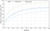 |
Fig. 5 Comparison of convergence curves of optimization algorithms. |
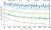 |
Fig. 6 Comparison of PSL performance of different arrays. |
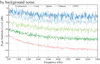 |
Fig. 7 Comparison of side-lobe levels at the full frequency band peak. |
5.2 Crack sound warning performance
Based on the array optimization, the recognition performance of AMAF-Net on the crack voiceprint warning task was further evaluated. Table 4 summarizes the comparison results of accuracy, precision, recall, F1 score and AUC between the proposed method and MFCC-SVM, WPE-RF and ResNet-18 baseline models on the test set.
AMAF-Net significantly outperformed the three categories of baseline methods on all five measures. Compared with ResNet-18, the AUC value of AMAF-Net was improved from 0.928 to 0.967 (p = 0.008), and the recall rate was improved from 0.862 to 0.913. The improvement of recall rate is particularly critical, because it is directly related to the missing report control of early cracks – in the scenario of preventive operation and maintenance, a missed report of crack growth may lead to several times the economic loss of false alarm. The improvement of recall rate of AMAF-Net is mainly due to two aspects. First, the dual attention mechanism enhances the focusing ability of the crack-sensitive frequency band, so that the network can capture weak voice-pattern components from strong background noise. Secondly, the contrast learning auxiliary task explicitly expands the separation degree of normal and crack cases in the feature space, and improves the inter-class boundary ambiguity problem [22].
Figure 8 shows the receiver operating characteristic curves and corresponding AUC values of each model. The ROC curve of AMAF‒Net was higher than that of the baseline model at all false positive rate levels, especially in the low false positive rate region (<0.1), indicating that the method could still maintain a high true rate under the premise of strict control of false positives. Based on the statistical results of 500 groups of threshold points, the average true rate of AMAF Net in the low false alarm area is 12.7% higher than Residual Network 18 (ResNet-18), and 28.3% higher than MFCC-SVM, which meets the demand of low false alarm and high reliable early warning in the wind field.
Figure 9 shows the loss decline curve of AMAF‒Net in the training process and the accuracy change curve of the verification set. It can be seen that the model basically converges around the 35th round, and there is no obvious over-fitting phenomenon. The training loss decreases rapidly from the initial 1.2 to below 0.1, and the accuracy of the validation set stabilizes above 0.93, which shows that the network has good fitting ability and generalization in the learning of crack voiceprint features. In 100 iterations, the maximum fluctuation of the accuracy of the validation set was less than 1.5%, and the stability of the model was better than that of the baseline DL method.
In order to visually compare the extraction and clustering effects of different methods on crack voiceprint features, t-SNE is used to reduce the high-dimensional features of all samples in the test set to two-dimensional space for visualization, and the results are shown in Figure 10. Where the green points represent the normal blade samples and the blue points represent the cracked blade samples. It can be seen from the figure that the feature distribution of MFCC SVM and WPE RF is highly overlapping, there is no obvious boundary between normal and crack samples, and the linear separability is poor. Although ResNet‒18 shows a certain clustering trend, the samples of small cracks are still scattered, and the discrimination between classes is limited. In the feature space of the AMAF‒Net network proposed in this paper, the two types of samples form an independent distribution with clear boundaries and compact clusters, and there is almost no overlap between normal and crack samples. It is fully verified that the double attention mechanism and contrast learning strategy can significantly enhance the discriminative feature expression of crack voiceprint. During the online monitoring phase, the average CPU inference time for AMAF-Net to process a single time-frequency feature map sample is approximately 35 ms on the Intel Xeon Gold 6226R CPU, which fully satisfies the real-time requirements for continuous wind turbine condition monitoring.
Performance comparison of different methods on the crack voiceprint warning task.
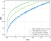 |
Fig. 8 Comparison of ROC curves of different methods. |
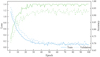 |
Fig. 9 Training loss and accuracy curve. |
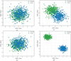 |
Fig. 10 t-SNE visualization of test set features for different methods. (a) MFCC-SVM, (b) WPE-RF, (c) ResNet18, (d) AMAF-Net. |
5.3 Ablation experiments
To systematically evaluate the contribution of each core module in CPSO-SM versus AMAF-Net, four ablation experiments were designed. Variant A removes the No-Refraction module of CPSO-SM, variant B removes the No-Surrogate mechanism, variant C removes the channel attention and temporal self-attention module of AMAF-Net, and variant C removes the No-Attention module of CPSO-SM. Variant D removes the loss of contrast learning AIDS (No-CL). Table 5 presents the performance degradation of each variant on the key metrics.
After removing the refractive correction of the shear layer, the NRMSE decreased from 0.104 to 0.158, with a relative increase of 51.9%, indicating that the physical correction of the propagation path had a decisive effect on the accuracy of the objective function of the array optimization. After removing the proxy model acceleration, the optimization process needed to directly call high-fidelity simulation due to the inability to quickly evaluate the candidate arrays in iterations. The training time skyrocketed to 47.6 hours, about 5.7 times of the full framework, which fully verified the key role of the Kriging proxy model in computational efficiency. Specifically, the average simulation time for a single high-fidelity acoustic case in COMSOL is approximately 45 min, while the surrogate-assisted optimization evaluates a candidate array in less than 0.02 seconds. Furthermore, the computational burden of CPSO-SM scales linearly rather than exponentially with the number of sensors, ensuring practical feasibility for expanding the array layout in industrial applications. After removing the attention mechanism, the AUC decreased from 0.967 to 0.941, and the recall decreased from 0.913 to 0.874, indicating that the dual attention design was indispensable for focusing the weak crack voiceprint components. After removing the contrastive learning loss, the AUC decreased to 0.949, and the recall rate of small crack cases decreased significantly, which verified the effectiveness of contrastive learning in enhancing the separability between classes.
Results of ablation experiments.
5.4 Case study
In order to further verify the applicability and interpretability of the proposed method in the actual scenario, a representative 20 mm crack sample in the test set was selected for in-depth analysis in this section. The sample was derived from the 8°-angle of attack condition of the wind tunnel experiment, and the incoming flow velocity is 35 m/s, which corresponds to the typical operating conditions of the fan blade tip region.
In order to quantify the improvement effect of the optimized array on the timeliness of warning, a typical sample of 20 mm cracks in the test set was selected to compare the timing response of the warning probability between the CPSO‒SM optimized array and the traditional Archimedean spiral array. The results are shown in Figure 11. In the figure, the black dashed line is the warning threshold τ = 0.65, the green curve is the warning probability of the optimized array, and the orange curve is the warning probability of the spiral array. In the early crack excitation stage (t = 4–6 s), the optimized array took the lead in capturing weak voiceprint anomalies with lower side bakes and higher spatial resolution, and the warning probability quickly exceeded the threshold at t =5 s. However, the traditional spiral array is affected by side lobe interference and signal attenuation, and the early warning probability is delayed until t = 9 s, and the overall lag is about 2s. The results directly prove that the array topology optimization can significantly advance the warning time of early cracks and provide more abundant response window for preventive operation and maintenance of wind power plants.
The case analysis revealed two findings with practical implications. First, the array acquisition quality has a direct impact on the timeliness of early warning - better array configuration can capture weak voiceprint anomalies earlier, and win valuable response Windows for operation and maintenance decisions. Second, the response of AMAF-Net to the sound pattern of crack is clearly physically interpretable: the jump in the warning probability is highly synchronized in time with the energy concentration at the crack location in the beam map, indicating that the network decision is not blindly dependent on statistical correlation, but a reasonable response to the real acoustic representation of the crack. This feature is of great value to improve the trust of the AI early warning system in the industrial site.
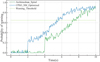 |
Fig. 11 Early warning process analysis of 20 mm crack samples. |
6 Discussion
6.1 Interpretation of results
The experimental results of this study show that the CPSO-SM optimized array is significantly better than the existing baseline methods in two dimensions of sound field reconstruction quality and crack warning performance. From an acoustically physical perspective, the root cause of this improvement is the explicit introduction of shear-layer refraction and column scattering correction in the array optimization process. The traditional free-field sparse optimization method assumes that the sound wave propagates along a straight line. However, in the actual wind field environment, the velocity gradient on both sides of the blade wake shear layer causes the acoustic ray to bend, which leads to systematic deviation in the time delay estimation based on the linear propagation assumption [4]. In this paper, the ray tracing method is used to modify the transfer function, so that the array manifold is consistent with the actual propagation path, and the main lobe offset and side lobe lift are effectively suppressed in beamforming. This finding is consistent with the conclusion of Xu review on the effect of shear layer on the accuracy of sound source localization, but the correction mechanism is systematically embedded in the array optimization closed loop, rather than as a post-processing compensation [6].
From the perspective of feature learning, the dual attention mechanism and contrastive learning strategy of AMAF-Net jointly improve the representation ability of weak crack voiceprint. The results of ablation experiments confirmed that the recall decreased most significantly after removing the attention module, indicating that the joint attention weighting of the channel and temporal dimensions is critical for screening the crack sensitive band from strong background noise. This echoes the comments of Gangsar on the effectiveness of attention mechanism in acoustic monitoring of rotating machinery, but this paper further introduces contrast learning into the training framework, and uses the embedding constraint that like attracts and different types repel to enhance the separation between normal and crack conditions in the feature space [17]. The t-SNE visualization clearly shows this effect – the learned features of AMAF-Net form a cluster structure with compact within class and separated between classes, which provides a geometric basis for high recall early warning.
The introduction of closed-loop joint optimization strategy contributes additional gains at the system level. By feeding the sensitivity gradient of the early warning network to the input SNR to the array coordinates, the array layout is not only pursuing the optimal acoustic imaging quality, but directly serving the performance improvement of the downstream early warning task. This design concept is consistent with the collaborative optimization framework of sensor layout and monitoring tasks advocated, but this paper is the first to land it in the field of fan blade voile-pattern monitoring, and an operational gradient approximation implementation scheme is given.
6.2 Limitations
Despite the encouraging experimental results of the proposed framework, several limitations remain to be improved in subsequent work. Firstly, the accuracy of sound field simulation depends on the accurate acquisition of the incoming wind speed profile and the pressure distribution on the blade surface. Although the Amiet trailing edge noise model used in this paper has good prediction accuracy in the medium Reynolds number range, no perfect correction model has been established for noise spectrum modulation caused by non-ideal factors such as blade surface roughness change and leading-edge erosion, which may lead to deviation between the simulated sound field and the actual field sound field. Secondly, the finite difference method is used to approximate the gradient in closed-loop joint training. Although the complex adjoint solver development is avoided, the computational overhead in high-dimensional array space cannot be ignored, especially when the number of sensors increases to tens of channels, the method is difficult to scale. Thirdly, the current validation is based on a wind tunnel controlled experimental dataset [17]. Although this dataset is representative in the field of blade acoustic monitoring, there are still differences in the turbulence degree and background noise characteristics between the coming flow and the open environment of a real wind farm. The generalization ability of the method on real wind turbines needs to be further tested. To ensure transferability to real wind farm environments, practical deployment will require site-specific field calibration. Future implementations must integrate operational SCADA data and employ transfer learning techniques to fine-tune the baseline model against variable atmospheric turbulence, complex terrain effects, and unpredictable mechanical background noise present in open environments. In addition, this paper only verified the typical damage mode of trailing edge crack, and the suitability of voice features for other types of damage, such as delamination and fiber fracture, has not been investigated.
6.3 Practical implications
This study has many guiding significances for the engineering practice of wind power plant blade acoustic monitoring system. At the hardware deployment level, the CPSO-SM algorithm provides a reusable array layout design tool. The operator only needs to input the geometric parameters and typical operating condition range of the target machine, and the algorithm can automatically output the optimized sensor coordinates without relying on the repeated debugging of acoustic experts. At the level of early warning strategy, the high recall of AMAF-Net effectively reduces the risk of missed crack report, which has direct economic value for modern wind farms where preventive operation and maintenance are the core cost control means. At the system integration level, the closed-loop joint training strategy shows that the co-design of the sensing front end and the recognition back end is an effective way to improve the overall performance of the monitoring system, rather than isolated optimization. This concept can be extended to other structural health monitoring modes such as guided wave and vibration.
6.4 Future work
Future research can be deepened along the following directions. Firstly, the completeness of the sound source model was extended, and high-fidelity noise source data based on boundary element (BEM) or large eddy simulation (LCE) was introduced to establish a voice pattern evolution database covering the whole blade life cycle (including leading edge erosion, trailing edge wear, etc.), so as to enhance the ability of the simulation model to describe the real degradation process. Secondly, the adjoint method is explored to replace the finite difference method to realize the accurate and efficient calculation of the gradient, so that the closed-loop joint training can be extended to large-scale 3D array optimization problems. Thirdly, the SCADA operation data and blade endoscopy records were combined to evaluate the robustness of the method under non-stationary wind conditions and complex terrain conditions, and the simulation and measured data transfer learning mechanism was established to bridge the field gap. Fourth, the single crack detection is extended to multiple damage concurrent recognition, and the voiceprint decouple network for multi-label classification is designed to improve the system's diagnostic ability for complex damage scenes.
7 Conclusion
This study established a closed-loop optimization framework, CPSO-SM and AMAF-Net, to address spatial aliasing and weak signal attenuation in wind turbine blade acoustic signature monitoring. By embedding shear-layer refraction physics into a surrogate-assisted particle swarm optimization process, the framework yields an array topology that demonstrably reduces the normalized root mean square error by 44.4% relative to conventional spiral arrays. The corresponding attention-based acoustic network achieved an area under the curve of 0.967 and a recall of 0.913 in identifying early-stage trailing-edge cracks.
The findings confirm that integrating multi-physics propagation constraints directly into the array optimization loop—rather than treating them as post-hoc corrections—is essential for preserving signal fidelity in complex wind farm environments. The proposed closed-loop strategy further reveals that optimizing the sensing front-end jointly with the diagnostic back-end mitigates the performance degradation typically observed in sequential design paradigms.
Beyond providing a reusable sensor layout tool for wind turbine towers and nacelles, this work establishes a methodological basis for extending cognitive-load-aware optimization to other simulation-intensive structural health monitoring tasks. Future extensions will explore gradient-adjoint methods for real-time array reconfiguration and the integration of this framework with digital twin platforms for predictive maintenance scheduling.
Funding
This research received no external funding.
Conflicts of interest
All authors declare that they have no conflicts of interest.
Data availability statement
This article has no associated data generated and/or analyzed.
Author contribution statement
Bihua Zou: Supervision, Writing—original draft; Jiefeng Liu: Methodology, Validation, Formal Analysis.
References
- P. Andrade, K. Laadjal, A.N. Alcaso et al., A comprehensive review on condition monitoring and fault diagnosis in fuel cell systems: challenges and issues, Energies, 17, 657 (2024) [Google Scholar]
- Y. Zhang, F. Avallone, S. Watson, Wind turbine blade trailing edge crack detection based on airfoil aerodynamic noise: an experimental study, Appl. Acoust. 191, 108668 (2022) [Google Scholar]
- Z. Rao, Multisource financial data fusion enhanced anomaly transaction detection and early-warning mechanism, Int. J. Inf. Commun. Technol. 26, 1–18 (2025) [Google Scholar]
- Z. Sun, W. Zhu, E. Jané et al., Sound propagation analysis of a 10 MW wind turbine: influence of the tower, operational states, and atmospheric conditions, Renew. Energy, 255, 123842 (2025) [Google Scholar]
- W. Xue, B. Yang, Aeroacoustic source localization using the microphone array method with application to wind turbine noise, Int. J. Aeroacoust. 23, 533–557 (2024) [Google Scholar]
- Q. Xu, H. Wang, Sound field modeling method and key imaging technology of an ultrasonic phased array: a review, Appl. Sci. 12, 7962 (2022) [Google Scholar]
- J. Zhang, Y. Wen, J. Yan et al., Improvement of orthogonal matching pursuit deconvolution beamforming method for acoustic source identification, J. Low Freq. Noise Vib. Act. Control, 42, 209–221 (2023) [Google Scholar]
- L. Brandetti, F. Avallone, D. De Tavernier et al., Assessment through high-fidelity simulations of a low-fidelity noise prediction tool for a vertical-axis wind turbine, J. Sound Vib. 547, 117486 (2023) [Google Scholar]
- Y. Teff-Seker, O. Berger-Tal, Y. Lehnardt et al., Noise pollution from wind turbines and its effects on wildlife: a cross-national analysis of current policies and planning regulations, Renew. Sustain. Energy Rev. 168, 112801 (2022) [Google Scholar]
- F. De Girolamo, L. Tieghi, G. Delibra et al., Sensitivity analysis of wind turbine broadband noise estimation to semi-empirical models parameters, J. Basic Appl. Sci. 19, 97–105 (2023) [Google Scholar]
- S. Saleh, T. Saeidi, N. Timmons et al., Overview of RF-based structural health monitoring of wind turbine blades, Front. Antennas Propag. 3, 1755037 (2025) [Google Scholar]
- C. Zhang, M. Wei, Coherence CLEAN-SC (C–CLEAN-SC) phased array processing for coherent sound source localization, Chin. J. Aeronaut. 38, 103500 (2025) [Google Scholar]
- J. He, Y. Xiao, C. Zhang et al., Deconvolution model for the cyclostationary acoustic source beamforming with high spatial resolution, Appl. Acoust. 242, 111085 (2026) [Google Scholar]
- C. Ocker, E. Blumendeller, P. Berlinger et al., Localization of wind turbine noise using a microphone array in wind tunnel measurements, Wind Energy, 25, 149–167 (2022) [Google Scholar]
- E. Nikolaou, S. Kilimtzidis, V. Kostopoulos, Multi-fidelity surrogate-assisted aerodynamic optimization of aircraft wings, Aerospace, 12, 359 (2025) [Google Scholar]
- Z. Li, Y. Zhao, Y. Zhang et al., A novel transformer-enhanced and acoustic-based approach for wind turbine blade fault detection with integrated system implementation, J. Eng. Des. 36, 642–671 (2025) [Google Scholar]
- P. Gangsar, A.R. Bajpei, R. Porwal, A review on deep learning based condition monitoring and fault diagnosis of rotating machinery, Noise Vib. Worldwide, 53, 550–578 (2022) [Google Scholar]
- S. Zhu, P. Chen, X. Li et al., MSRDSN: a novel deep learning model for fault diagnosis of high-voltage disconnectors, Electronics, 14, 4151 (2025) [Google Scholar]
- G. Zhong, Deep learning and layered architecture-based anomaly detection method for IoT, Int. J. Inf. Commun. Technol. 26, 52–66 (2025) [Google Scholar]
- A. Van Biesbroeck, F. Shang, D. Bassir, CAD model segmentation via deep learning, Int. J. Comput. Methods, 18, 2041005 (2020) [Google Scholar]
- F. Yi, R. Zhong, W. Zhu et al., Leakage fault diagnosis of wind tunnel valves using wavelet packet analysis and vision transformer-based deep learning, Mathematics, 13, 3195 (2025) [Google Scholar]
- Y. Liu, Electronic component fault diagnosis based on cross-domain features and deep contrastive learning, Int. J. Inf. Commun. Technol. 26, 92–110 (2025) [Google Scholar]
Cite this article as: Bihua Zou, Jiefeng Liu, Optimization and early warning strategy for wind turbine blade acoustic signature monitoring array based on wind farm simulation, Int. J. Simul. Multidisci. Des. Optim. 17, 16 (2026), https://doi.org/10.1051/smdo/2026012
Appendix
A
Input: Initial DoE samples  , total budget B, maximum iterations Tmax
Output: Optimized array configuration 
1. Initialize Kriging model  with D
2. Initialize particle swarm 
3.  ,
, 
4. while  and
and  do
do
5. for each particle i = 1 to Np do
6. 
7.  DiscreteUpdate (Xi, Vi)
8. 
9. 
10. Update  and
and 
11. end
12. Compute EI criterion: 
13. 
14.  Acoustic Simulation (
 )
)
15. 
16. Update  with augmented D
17. 
18. if  then
then
19. break
20. 
21: end
22. return Gbest
All Tables
Comparison of acoustic field reconstruction performance for different array configurations.
Performance comparison of different methods on the crack voiceprint warning task.
All Figures
|
Fig. 1 Overall architecture and data flow of the proposed CPSO-SM and AMAF-Net joint optimization framework. |
| In the text | |
|
Fig. 2 Architecture of multi-physics acoustic propagation modeling. |
| In the text | |
|
Fig. 3 CPSO-SM collaborative architecture. |
| In the text | |
|
Fig. 4 AMAF-Net architecture. |
| In the text | |
|
Fig. 5 Comparison of convergence curves of optimization algorithms. |
| In the text | |
|
Fig. 6 Comparison of PSL performance of different arrays. |
| In the text | |
|
Fig. 7 Comparison of side-lobe levels at the full frequency band peak. |
| In the text | |
|
Fig. 8 Comparison of ROC curves of different methods. |
| In the text | |
|
Fig. 9 Training loss and accuracy curve. |
| In the text | |
|
Fig. 10 t-SNE visualization of test set features for different methods. (a) MFCC-SVM, (b) WPE-RF, (c) ResNet18, (d) AMAF-Net. |
| In the text | |
|
Fig. 11 Early warning process analysis of 20 mm crack samples. |
| In the text | |
Current usage metrics show cumulative count of Article Views (full-text article views including HTML views, PDF and ePub downloads, according to the available data) and Abstracts Views on Vision4Press platform.
Data correspond to usage on the plateform after 2015. The current usage metrics is available 48-96 hours after online publication and is updated daily on week days.
Initial download of the metrics may take a while.