")
")
| Issue |
Int. J. Simul. Multidisci. Des. Optim.
Volume 10, 2019
|
|
|---|---|---|
| Article Number | A6 | |
| Number of page(s) | 9 | |
| DOI | https://doi.org/10.1051/smdo/2019007 | |
| Published online | 21 March 2019 | |
Research Article
Current correction and fuzzy logic optimizations of Perturb & Observe MPPT technique in photovoltaic panel
Laboratory of Innovative Technologies, National School of Applied Sciences, Abdelmalek Essaâdi University, 93030 Tangier, Morocco
* e-mail: This email address is being protected from spambots. You need JavaScript enabled to view it.
Received:
29
December
2017
Accepted:
17
February
2019
Abstract
This paper presents a two-way optimization of the Perturb & Observe (P&O) maximum power point tracking (MPPT) technique using current correction and fuzzy logic techniques. In fact, photovoltaic (PV) energy has become more and more coveted today. In the future, it will become a necessity. To ensure its optimization, maximum operating point tracking method is considered as a technological key in PV systems. One of the most used MPPT methods is the P&O technique. In this paper, we will focus on optimizing this method based on two techniques. A first attempt has been made to estimate a current correction of the P&O algorithm in case of illumination variation. Then, fuzzy logic optimization attempt had been highlighted to improve power loss. It is shown that both proposed techniques are very effective and allow considerable improvement of accuracy and are less affected by sudden variation of climatic parameters. The proposed approaches are tested via Matlab software and compared the classical P&O algorithm. Through applications, we could conclude that the two optimized proposed methods offer a remarkable improvement concerning power losses.
Key words: MPPT / Perturb & Observe algorithm / Fuzzy logic / Current correction / Photovoltaic energy
© M. Ourahou et al., published by EDP Sciences, 2019
 This is an Open Access article distributed under the terms of the Creative Commons Attribution License (http://creativecommons.org/licenses/by/4.0), which permits unrestricted use, distribution, and reproduction in any medium, provided the original work is properly cited.
1 Introduction
Faced with the depletion of fossil energy, solar energy provided by photovoltaic (PV) panels is an inexhaustible energy, reliable, easy to use, and especially respects nature and environment. Several researches have been developed since centuries through modeling techniques for renewable energy including PV systems. The aim is to develop opportunities for future investment and economic feasibility. Moreover, this energy remains the most “elegant” since it is silent and easily integrated into housing. However, PV energy production is nonlinear and varies depending on factors such as the illumination, the temperature, and the age of the panel itself. Therefore, operating point of the PV panel is often not coinciding with the maximum power point (MPP). So, the challenge is to, constantly, determine the maximum operating point of the PV panel in order to assign a maximum power to the load at all times. Indeed, the power generated by a PV panel depends on its operating voltage. Thus, the characteristic curves V–I and V–P specify a single point where the maximum power is delivered. This method is called maximum power point tracking (MPPT) [1,2]. To increase the efficiency of this method, we insert a regulation system on the PV panel that makes it a “follower” and allows us to optimize the electricity production depending on the type of sensors used, speed, efficiency, price, and accuracy.
Because the illumination and temperature levels clearly influence the operation at maximum power of the PV panel, this was the starting point for various techniques of MPPT. In this paper, we focus on the “Perturb & Observe” (P&O) method. In fact, when irradiation changes rapidly, the MPP drifts since the load is changing after each perturbation, and therefore the P&O method used loses its effectiveness [3]. This constitutes a niche for the first optimization technique which will be developed in the present paper. Afterward, another technique for optimizing the P&O method based on fuzzy logic will be highlighted. The aim of this second technique is to make a correction of the classic P&O method. Finally, a comparison between the two methods is made in order to determine which is the most effective.
The paper is organized as follows: Section 2 presents a mathematical model of a photovoltaic generator (PVG), Section 3 is devoted to the optimization techniques, Section 4 deals with the results and discussion, and Section 5 presents a summary of the results.
2 Photovoltaic generator mathematical model
A PVG is composed of several PV cells mounted in series and/or in parallel. It is also composed of a conversion system (DC-DC converter), MPPT controller, and storage device (DC load). This set is called a PV system and is shown in Figure 1. In fact, PV panel is the result of conversion of energy that photons carry from light when they are in contact with suitably processed semiconductor materials. When the incident light communicates energy to the semiconductor's electrons, some of them exceed the potential barrier. They are thus expelled to an external circuit [4,5].
Figure 2 shows the photovoltaic cell electrical model.
According to the Shockley equation: I d = I 0 (exp (e.V d/K.T)−1)
And: V d = (K.T/e). ln (I d/I 0 + 1).
Also, when the circuit to the terminals of the cell is opened: V 0c = (K.T/e). ln (I cc/I 0 + 1).
The parallel current which passes through the R p resistance is: I R = V d/R p.
Taking into account the effect of the series resistance, we have: V d = V + R s.I.
The final equation of PV panel model is: I = I cc−I 0 (exp (e.[V + R s.I]/K.T)−1) − ([V + R s.I]/R p).
Figure 3 explicates the characteristics of power–voltage (P–V) and current–voltage (I–V) of a PV panel using Simulink interface of Matlab software. This panel model is composed of 12 solar cells in series as shown in Table 1.
The MPP differs depending on temperature and illumination [6–9]. Indeed, Figure 4 shows current curves variations for a steady temperature of 25 °C and different illuminations of 1000 W/m2, 600 W/m2, and 300 W/m2. Also, once illumination remains steady at 1000 W/m2 and temperature changes, from 300 K to 360 K, MPP varies considerably.
Conversion system is based on a BOOST type DC–DC converter. Figure 5 shows the electrical structure of this converter. The purpose of this converter is to realize an adaptation lift source–load between input and output voltage (V e and V s) [10].
At time t = 0, the transistor is closed. For a time t between 0 and αT, we have:
V e = L di/dt.
So:
The current curve is thus a growing curve based on the value I 1.
At the moment αT, the transistor is opened. For a time t between αT and period T, we have:
So,
For the BOOST converter, V s is always higher than V e. The power curve is decreasing starting from I 2 current value. Current curve during period T is then shown in Figure 6.
If the BOOST converter is in continuous conduction and its performance is ideal, we deduce that the adaptation between the source and the load depends on the duty cycle. Indeed, the voltage V
s can be expressed according to the voltage V:
By varying the duty cycle α, we can act on the load in such a way to maximize the power delivered by the PV panel. This is the main interest of the MPPT commands.
 |
Fig. 1 Photovoltaic cell cross-section and conversion elementary chain controlled by an MPPT controller. |
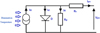 |
Fig. 2 Electrical model of photovoltaic cell. |
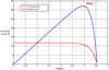 |
Fig. 3 Power–voltage (P–V) and current–voltage (I–V) characteristics. |
PV panel characteristics.
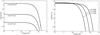 |
Fig. 4 I–V photovoltaic panel characteristics under different climate conditions. |
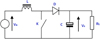 |
Fig. 5 Electrical structure of the BOOST converter. |
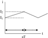 |
Fig. 6 Current curve for a BOOST converter. |
3 Optimization techniques
3.1 Perturb & Observe method
MPPT method is a mechanism that ensures instantaneous adaptation of the load operating point to the power supplied by the PVG. A distinction is made between direct and indirect research methods:
-
Direct MPPTs operate through currents, voltages, or power measurements directly on the system. This ensures the reaction in case of unpredictable changes.
-
Indirect MPPTs operate through the measured values and the approximate position of the MPP.
Among the MPPT commands, P&O is one of the most used commands because of its simple structure and the reduced number of parameters to control [11].
The principle is to generate disturbances by reducing or increasing the duty ratio D and to observe the effect of the generated power by the PV panel. Once the periodic V the voltage disturbance of the panel is done, it can decide on the next cycle [12–14]. It is also important to note that the disturbance ΔV is low so that the power variation is not too excessive. Thus, if:
-
dP/dV > 0, we approach the MPP and the perturbation moves the operating point closer to the MPP. The cyclic ratio variation in the same direction is thus maintained until the MPP has been reached.
-
dP/dV < 0, we move away from the MPP and the perturbation moves the operating point farther from the MPP. The cyclic ratio variation must be done in the opposite direction until reaching the MPP.
-
dP/dV = 0, we are at the MPP.
For this method there is a compromise between accuracy and speed since the disturbance must be very low so that the power change is not too big and thus minimize power losses [15,16]. The controller based on the P&O algorithm has two input values that are measured constantly, which are the current and the voltage. From these measurements, it calculates the power P, the voltage variation ΔV, and the power variation ΔP between K and K−1 iterations as shown in Figure 7.
The output power of a PVG depends on the received irradiation. Indeed, the voltage does not vary considerably contrary to current that increases strongly.
In this case, the solution would be to make a control loop not only over voltage and power but also over the current. It allows to control permanently current variation and thus to identify as much as possible any variation of illumination. In fact, at each instant k, the PV panel has a characteristic I–V. These two parameters are measured continuously at the input of each cycle. Thus, instead of calculating only voltage and power variations V and P, we also calculate the variation of the current I. This will reflect any eventual insolation variation at the cycle input. Where applicable, this will be a new characteristic I–V of the PV panel. So, the algorithm can act directly on the duty cycle to correct this drift, to regain control of power and voltage, and therefore to go back to the classic maximum operating point tracking.
Indeed, in a classic P&O algorithm, the value of current I measured at panel output is never stable and varies within a range of absolute value lower than a limit L as [17]:
In order to make the algorithm insensible to these current changes due to the oscillation, we will set a threshold S higher than the limit L. It will allow to test insolation variation. Therefore, we take a value S > L.
So if:
-
│i(k)−i(k − 1)│ < S, the algorithm is a classic P&O algorithm that has not gone through any insolation variation.
-
│i(k)−i(k − 1)│ > S, the PV panel has gone through an insolation variation. That gives a new characteristic curve I–V. And the algorithm acts directly on the cyclic ratio.
The operating direction depends on the sign of the current variation I. In fact, if:
-
I > 0, so the insolation variation has increased and the voltage must then be incremented by V.
-
I < 0, so the insolation variation has decreased and the voltage must be decremented by V.
Figure 8 presents the proposed optimized P&O algorithm with current correction.
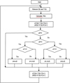 |
Fig. 7 Perturb & Observe classic algorithm. |
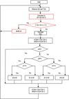 |
Fig. 8 Optimized Perturb & Observe algorithm. |
3.2 Fuzzy logic method
The world that surrounds the human being is full of uncertainties and inaccurate perceptions. By nature, man incorporates certain imperfections in everyday life, particularly while reasoning and deciding. The idea is to define a multivalued logic allowing to model these imperfections and to take into account the intermediate states between “all” and “nothing.” In this perspective, a fuzzy controller does not require a system model to be set. The adjustment of algorithms is based on linguistic rules such as: as if … Then … In fact. These rules can be expressed using everyday language and the intuitive knowledge of a human operator.
In our application case, fuzzy logic is a method that will allow the reduction of error without the need for an exact knowledge of system mathematical model. The fuzzy controller is divided into three essential steps − fuzzification, inference, and defuzzification − as shown in Figure 9 [18–20].
-
Fuzzification
Fuzzification consists on converting physical variables inputs into fuzzy sets, which is based on a membership degree for each input.
-
Inference
This is where decisions are made. The inference uses rules for determining the output signal of the controller as a function of the input signals [21–23].
In these, rules intervene the operators AND and OR. The AND operator is applied inside a rule to link the variables. And the OR operator is applied outside the rules to link them. There are several methods of inference such as MAX-MIN method, MAX-PROD method, and SUM-SPROD method. In our application case, the MAX-MIN inference method is used which realizes the AND operator for the minimum and the operator OR for the maximum.
For the conclusion, the operator THEN links the output variable with the degree of membership of the input variable.
-
Defuzzification
This step allows to convert the fuzzy output variables at the end of inference step into adapted physical variables. There are several methods of defuzzification such as the maximum method, the weighted average method, and the centroid method (the so-called center of gravity). In this paper, the last method was used [24,25].
The input variables for the fuzzy controller are the power and the voltage variations.

We consider three intervals for the inputs V, P, and the output dD:
-
P: Positive;
-
Z: Zero;
-
N: Negative.
The membership functions of the output and the two inputs are shown in Figures 10–12.
The inference rules of this controller are derived from the classic P&O algorithm. Indeed, according to Figure 7, it can be deduced that:
-
If P is zero, so we are in PMP point and there is no variation of the duty cycle (dD is zero).
-
If P and V have the same sign, so the duty cycle is increased (dD is positive).
-
If P and V have opposite sign, so the duty cycle is decreased (dD is negative).
In the world of fuzzy logic, the following rules of inference can be stated:
-
If P is “P” and V is “P” then dD is “N” (if P is positive and V is positive then dD is negative).
-
If P is “P” and V is “Z” then dD is “Z” (if P is positive and V is zero then dD is zero).
-
If P is “P” and V is “N” then dD is “P” (if P is positive and V is negative then dD is positive).
-
If P is “N” and V is “P” then dD is “P” (if P is negative and V is positive then dD is positive).
-
If P is “N” and V is “Z” then dD is “Z” (if P is negative and V is zero then dD is zero).
-
If P is “N” and V is “N” then dD is “N” (if P is negative and V is negative then dD is negative).
-
If P is “Z” and V is “P” then dD is “Z” (if P is zero and V is positive then dD is zero).
-
If P is “Z” and V is “Z” then dD is “Z” (if P is zero and V is zero then dD is zero).
-
If P is “Z” and V is “N” then dD is “Z” (if P is zero and V is negative then dD is zero).
These new fuzzy rules can be integrated in Table 2.
 |
Fig. 9 Steps of fuzzy logic controller. |
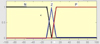 |
Fig. 10 Voltage variation membership function. |
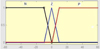 |
Fig. 11 Power variation membership function. |
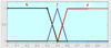 |
Fig. 12 Output membership function. |
Inference table.
4 Results and discussion
4.1 Current correction method
The simulations for both classic and improved P&O algorithms are performed in the same conditions: a temperature of 25 °C and a variable illumination.
The power behavior for these two cases is shown in Figure 13.
Figure 12 shows the power variation of the PV module depending on illumination variation. In fact, the improved algorithm has better response in the event of sudden insolation variation. Power loss in the case of P&O classic algorithm is P1. And, in the case of P&O optimized algorithm, the power loss is P2. By using optimization by current correction, we are able to gain in terms of PV panel power in case of illumination variation.
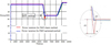 |
Fig. 13 Power variation and power loss for each algorithm. |
4.2 Fuzzy logic method
The simulations for both classic and fuzzy logic improved P&O algorithms is performed in a temperature of 25 °C and an illumination of 1000 W/m2 (Fig. 14).
Both power curves have the same shape especially in terms of speed and stability. However, the optimized method power curve is more precise. Next, we vary the illumination while keeping the temperature fixed at 25 °C (Fig. 15).
The classic P&O algorithm curve was affected by the sudden change of illumination since the P&O improved algorithm behavior is more accurate.
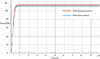 |
Fig. 14 Power curve for fixed climatic parameters. |
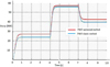 |
Fig. 15 Power curve for fixed temperature and variable illumination. |
5 Conclusion
PVG system based on a P&O algorithm has been presented. The mathematical model was developed based on a one diode model and a boost convertor. This paper discussed two different optimization algorithms of the classic P&O method: current correction and fuzzy logic to improve the efficiency of the system at different climate conditions especially illumination and temperature.
The simulated results show that both methods offer a remarkable improvement concerning power losses and precision. Comparison indicates that proposed models are effectives and accurate, and are less affected by sudden variation of climatic parameters.
From the simulation study, it has been found that fuzzy logic P&O optimized algorithm converges to the global optimum.
Nomenclatures
R s : Line contact resistance
R p, I R : Resistance and leakage current due to diode and effects on the junction
I G : Current created by absorbed solar radiation. It is practically worth the short circuit current I cc
(I PV, V PV): Photovoltaic panel characteristics
I 0 : Reserve saturation current
e : Charge of electrons
K : Boltzmann constant
T : Temperature
W : Illumination
a : Duty cycle
References
- X. Liu, An improved perturbation and observation maximum power point tracking algorithm for PV panels, thesis presented for the Degree of Master of Applied Science, Concordia University, Montreal, Quebec, Canada, 2004 [Google Scholar]
- A. Pradeep Kumar Yadav, S. Thirumaliah, G. Haritha, Comparison of MPPT algorithms for DC-DC converters based PV systems, Int. J. Adv. Res. Electr. Eectron. Instrum. Eng. 1 , 476 (2012) [Google Scholar]
- K.H. Hussein, T. Hashino, Maximum photovoltaic power tracking: an algorithm for rapidly changing atmospheric conditions, IEE Proc. Gener. Transm. Distrib. 142 , 59–64 (1995) [Google Scholar]
- B. Subudhi, R. Pradhan. A comparative study on maximum power point tracking techniques for photovoltaic power systems, IEEE Trans. Sustain. Energy 4 , 89–98 (2013) [CrossRef] [Google Scholar]
- S. Lyden, M.E. Haque, A. Gargoom, M. Negnevitsky, Review of maximum power point tracking approaches suitable for PV systems under partial shading conditions, in: Proceedings of the Australasian Universities Power Engineering Conference , Hobart, TAS, Australia, 2013, pp. 1–6 [Google Scholar]
- K. Ishaque, Z. Salam, A review of maximum power point tracking techniques of PV system for uniform insolation and partial shading condition, Renew. Sustain. Energy Rev. 19 , 475–488 (2013) [CrossRef] [Google Scholar]
- H.J. El-Khozondar, R.J. El-Khozondar, K. Matter, T. Suntio, A review study of photovoltaic array maximum power tracking algorithms, Renew. Wind Water Sol. 3 , 3 (2016) [CrossRef] [Google Scholar]
- A. Soufyane Benyoucef, A. Chouder, K. Kara, S. Silvestre, O.A. Sahed, Artificial bee colony based algorithm for maximum power point tracking (MPPT) for PV systems operating under partial shaded conditions, Appl. Soft Comput. 32 , 38–48 (2015) [CrossRef] [Google Scholar]
- A. Elnosh, V. Khadkikar, W. Xiao, J.L. Kirtely, An improved extremum-seeking based MPPT for grid-connected PV systems with partial shading, in: 2014 IEEE 23rd International Symposium on Industrial Electronics , Istanbul, Turkey, 2014, pp. 2548–2553 [Google Scholar]
- G.M. Masters, Renewable and efficient electric power systems (John Wiley & Sons, Inc., Hoboken, NJ, 2004) [CrossRef] [Google Scholar]
- R.W. Erickson, DC-DC power converters, in: Wiley Encyclopedia of Electrical and Electronics Engineering (John Wiley & Sons, NY, 2007) [Google Scholar]
- M. Lokanadham, K. Vijaya Bhaskar, Incremental conductance based maximum power point tracking (MPPT) for photovoltaic system, Int. J. Eng. Res. Appl. 2 , 1420–1424 (2012) [Google Scholar]
- Salazar, F. Tadeo, C. Prada, L. Palacin, Simulation and control of a PV system connected to a low voltage network, Jornadas De Automática, 8–10 September 2010, Jaén, Spain [Google Scholar]
- N. Femia, G. Petrone, G. Spagnuolo, M. Vitelli, Optimization of perturb and observe maximum power point tracking method, IEEE Trans. Power Electron. 20 , 963 (2005) [Google Scholar]
- A. Chermitti, O. Boukli-Hacene, S. Mouhadjer, Design of a library of components for autonomous photovoltaic system under Matlab/Simulink, Int. J. Comput. Appl. 53 , 13–19 (2012) [Google Scholar]
- R.J. Wai, W.H. Wang, C.Y. Lin, High-performance stand-alone photovoltaic generation system, IEEE Trans. Ind. Electron. 55 , 240–250 (2008) [CrossRef] [Google Scholar]
- C. Hua, J. Lin, An on-line MPPT algorithm for rapidly changing illuminations of solar arrays, Renew. Energy 28 , 997–1157 (2003) [CrossRef] [Google Scholar]
- A. Harrag, S. Messalti, How fuzzy logic can improve PEM fuel cell MPPT performances?, Int. J. Hydrogen Energy 43 , 537 (2017) [CrossRef] [Google Scholar]
- A. Harrag, H. Bahri, Novel neural network IC-based variable step size fuel cell MPPT controller: performance, efficiency and lifetime improvement, Int. J. Hydrogen Energy 42 , 3549e63 (2017) [CrossRef] [Google Scholar]
- N.H. Saad, A.A. El-Sattar, A.M. Mansour, Adaptive neural controller for maximum power point tracking of ten parameter fuel cell model, J. Electr. Eng. 13 , 1e7 (2013) [Google Scholar]
- R.W. Erickson, Fundamentals of power electronics (Chapman & Hall, New York, 1997) [CrossRef] [Google Scholar]
- J. Prakash, S.K. Sahoo, S.P. Karthikeyan, I.J. Raglend, Design of PSO-fuzzy MPPT controller for photovoltaic application power electronics and renewable energy systems (Springer, India, 2015), pp. 1339–1348 [Google Scholar]
- K. Premkumar, B.V. Manikandan, Adaptive neuro-fuzzy inference system based speed controller for brushless DC motor, Neurocomputing 138 , 260–270 (2014) [CrossRef] [Google Scholar]
- A. Chaouachi, R.M. Kamel, K. Nagasaka, A novel multi-model neuro-fuzzy-based MPPT for three-phase grid-connected photovoltaic system, Sol. Energy 84 , 2219–2229 (2010) [CrossRef] [Google Scholar]
- C. Larbes, S.A. Cheikh, T. Obeidi, A. Zerguerras, Genetic algorithms optimized fuzzy logic control for the maximum power point tracking in photovoltaic system, Renew. Energy 34 , 2093–2100 (2009) [Google Scholar]
Cite this article as: Meriem Ourahou, Wiam Ayrir, Ali Haddi, Current correction and fuzzy logic optimizations of Perturb & Observe MPPT technique in photovoltaic panel, Int. J. Simul. Multidisci. Des. Optim. 10, A6 (2019)
All Tables
All Figures
|
Fig. 1 Photovoltaic cell cross-section and conversion elementary chain controlled by an MPPT controller. |
| In the text | |
|
Fig. 2 Electrical model of photovoltaic cell. |
| In the text | |
|
Fig. 3 Power–voltage (P–V) and current–voltage (I–V) characteristics. |
| In the text | |
|
Fig. 4 I–V photovoltaic panel characteristics under different climate conditions. |
| In the text | |
|
Fig. 5 Electrical structure of the BOOST converter. |
| In the text | |
|
Fig. 6 Current curve for a BOOST converter. |
| In the text | |
|
Fig. 7 Perturb & Observe classic algorithm. |
| In the text | |
|
Fig. 8 Optimized Perturb & Observe algorithm. |
| In the text | |
|
Fig. 9 Steps of fuzzy logic controller. |
| In the text | |
|
Fig. 10 Voltage variation membership function. |
| In the text | |
|
Fig. 11 Power variation membership function. |
| In the text | |
|
Fig. 12 Output membership function. |
| In the text | |
|
Fig. 13 Power variation and power loss for each algorithm. |
| In the text | |
|
Fig. 14 Power curve for fixed climatic parameters. |
| In the text | |
|
Fig. 15 Power curve for fixed temperature and variable illumination. |
| In the text | |
Current usage metrics show cumulative count of Article Views (full-text article views including HTML views, PDF and ePub downloads, according to the available data) and Abstracts Views on Vision4Press platform.
Data correspond to usage on the plateform after 2015. The current usage metrics is available 48-96 hours after online publication and is updated daily on week days.
Initial download of the metrics may take a while.