© H.J. Bukhari, published by EDP Sciences, 2017

1 Introduction

Robust design optimization methods refers to a class of methods that can accommodate uncertainty while maintaining feasibility. The uncertainty in data is accommodated by accepting suboptimal solutions to a nominal design optimization problem. This methodology ensures that the design solution remains feasible and close to optimal even if there is a change in data. Different methodologies for robust design and optimization in mechanical systems have been extensively discussed in literature [1–14]. Most of these methods assume some kind of distribution for the uncertain variable to optimize the problem.

Most systems in practice are designed deterministically so that they are optimal with respect to certain variables that are assumed to operate strictly under designed conditions. Normal optimization routines either maximize or minimize an objective function given some constraints placed on the problem so that the system is optimal only when the design conditions are met completely. But design variables are inherently stochastic and the environment that they are designed to operate in is uncertain. The uncertainties in the operating environment are introduced from a variety of sources including manufacturing errors and incomplete information about the nature of the problem.

Therefore it is prudent to optimize design based on uncertainties that might be encountered by the system. Robust designs are able to meet design objectives while taking into account aberrations that might affect the system. Such designs are generally suboptimal with respect to the deterministic design but are robust under design uncertainties. The fundamental principle of robust design is to improve product quality or stabilize performances by minimizing the effects of variations without eliminating their causes [15]. Usually sensitivity analysis is done after the optimization procedure to ascertain the affect of change of one or more variables on the objective function. On the contrary robust design methodology accommodate uncertainty during the design process itself by making sure that the design remains feasible when subject to variation. Hence, reducing the possibility of large scale design changes after the design has been fielded.

2 Robust optimization framework

2.1 Linear robust optimization

Most robust design methods only take implementation errors into account by assuming a certain distribution for design variables but ignore parametric uncertainties. Implementation errors generally arise because of fabrication errors while parametric uncertainties are caused by noises in the system that have not been accounted for or missing variables that were not considered in the design. In actual environments parameters are subject to uncertainty as well. Robust solutions guarantee near optimal performance even if the optimum design is not realized. This means that a system designed using robust optimization will perform better than a deterministically designed system under non-ideal environment.

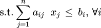
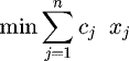
Consider the following linear optimization problem: $$\text{min}{\displaystyle \sum _{j=1}^n{c}_j{x}_j}$$ $$\text{s.t.}{\displaystyle \mathit{\sum }_{\mathit{j}\mathit{=}\mathit{1}}^{\mathit{n}}{\mathit{a}}_{\mathit{i}\mathit{j}}\mathit{}{\mathit{x}}_{\mathit{j}}}\le b_i,\forall i$$(1) $$l_j\le x_j\le u_j,\forall j$$

Assume that only the parameter values of matrix A are uncertain i.e., a_ij are uncertain parameters belonging to a known uncertainty set.

Reference [16] considers column wise uncertainty in matrix A and gives a robust formulation of problem (1) as follows $$\text{min}\underset{}{\overset{}{{\displaystyle \sum _{j=1}^n{c}_j{x}_j}}}$$ $$\text{s.t.}\underset{}{\overset{}{{\displaystyle \sum _{j=1}^n{a}_{ij}{x}_j}}}+{\displaystyle \sum _{j\in J_i}^n{\widehat{\mathit{a}}}_{ij}{y}_j}\le b_i,\forall i$$ $$-y_j\le x_j\le y_j$$(2) $$l_j\le x_j\le u_j,\forall j$$ $$y_j\ge 0$$

Robust optimization can be thought of as a worst-case minimization algorithm. The optimal decision is to protect against worst case scenarios by taking values from within the parameter bound set χ.

Reference [17] gives an alternative formulation of robustness for problem (1) by introducing a concept of price of robustness where assuming the uncertain parametersã_ij to be symmetric and bounded variables and j ∈ J_i be the set of coefficients subject to parameter uncertainty that assume values in the interval . They introduce a parameter Γ_i, not necessarily an integer, that takes values in the interval . The role of Γ_i is to adjust the robustness of the model against the level of conservatism of the solution. The budget of uncertaintyputs a limit on the number of constraints that can deviate from their mean : , Γ = 0 means that and return to the nominal problem (1). On the other hand if Γ = ∣J_i∣, this makes the constraint redundant where ∀i which makes the constraint very conservative (Soyster’s approach). And if Γ ∈ [0, n] we can adjust the degree of robustness of the problem and hence put a limit on the number of parameters that can be at their worst-case values simultaneously. The objective is to allow change of only up to coefficients so that one coefficient a_it changes by . $$\text{max}{c}^{\prime }x$$ $$\text{s.t.}\underset{}{{\displaystyle \sum _{\mathit{j}}^{}{\mathit{a}}_{\mathit{i}\mathit{j}}\mathit{}{\mathit{x}}_{\mathit{j}}}}\underset{S_i\cup \left\{t_{{}_i}\right\}|S_i\subseteq J_i,\left|S_i\right|=\lfloor {\Gamma }_i\rfloor ,t_i\in J_i\backslash S_i}{\text{max}}$$ $$\left\{{\displaystyle \sum _{\mathit{j}\in S_i}^{}{\widehat{a}}_{\mathit{i}\mathit{j}}{\mathit{y}}_{\mathit{j}}}+\left({\Gamma }_i-\lfloor {\Gamma }_i\rfloor \right){\widehat{a}}_{i{t}_i}{y}_t\right\}\le b_i\forall i$$(3) $$-y_j\le x_j\le y_j\forall j$$ $$l\le x\le u$$ $$y\ge 0$$

Reference [17] also provide an alternative formulation (4). So the classical approach of (2) can be transformed into $$\text{max}{c}^{\prime }x$$ $$\text{s.t.}{\displaystyle \sum _{\mathit{j}}^{}{a}_{ij}{x}_j}+z_i{\Gamma }_i+{\displaystyle \sum _{\mathit{j}\in J_i}^n{p}_{ij}}\le b_i\forall i$$ $$z_i+p_{ij}\ge {\widehat{\mathit{a}}}_{ij}{y}_j\forall i,j\in J_i$$ $$-y_j\le x_j\le y_j\forall j$$ $$l_j\le x_j\le u_j\forall j$$(4) $$p_{ij}\ge 0\forall i,j\in J_i$$ $$y_j\ge 0\forall j$$ $$z_i\ge 0\forall i$$

2.1.1 Example: Robust Air Cleaner Design

Let us apply this formulation to a practical problem illustrated below.

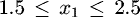
This problem is about a tractor manufacturing firm which wants to produce air cleaners for their tractors [18]. The schematic for the design is shown in Figure 1. The objective is to produce as many air cleaners per month as possible. The variables are the diameters of the exhaust duct x₁ and the main body x₂. The area of metal required by each air cleaner is given by $$1.6\left(2.75\pi x_1+10\pi x_2\right)$$

The dimensional constraints for the design are: $$1.50\le x_1\le 2.50$$ $$3.75\le x_2\le 6.25$$

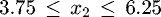
Another requirement is that the area of each cleaner should be at least 250 square inches; thus, $$1.6\left(2.75\pi x_1+10\pi x_2\right)\ge 250$$

The number of air cleaners to be produced is constrained by the amount of sheet metal that is available (15,000 square inches). The constraint on production level is that at least 50 cleaners need to be produced. Therefore, $$50\times 1.6\left(2.75\pi x_1+10\pi x_2\right)\le 15,000$$

Based on the robust formulation of equation (4), a robust linear problem that takes into account the uncertainty in the length of the exit duct (Γ₁ = 1) within 10% is as follows: $$\text{max}-\left(13.84x_1+50.24x_2\right)$$ $$\text{s.t.}-\left(13.84x_1+50.24x_2\right)+z_1{\Gamma }_1+P_{11}\le -250$$ $$690x_1+2510x_2+z_2{\Gamma }_1+P_{21}\le 15000$$ $$z_1+P_{11}\ge 1.38y_1$$ $$z_2+P_{21}\ge 69.0y_2$$(5) $$-y_1\le x_1\le y_1$$ $$1.5\le x_1\le 2.5$$ $$P_{11},P_{21}\ge 0$$ $$y_1,y_2\ge 0$$ $$z_1,z_2\ge 0$$

The solution of the above robust program gives an optimal value of 252.31, which is slightly worse off than the deterministic optimal of 250.24. A similar robust linear program can be written for inclusion of uncertainty in the length of the main body. The plots for this analysis are provided in Figure 2.

When Γ = 2, we return to Soyster’s formulation (2) which gives the following $$\text{max}-\left(13.84x_1+50.24x_2\right)$$ $$\text{s.t.}-\left(13.84x_1+50.24x_2\right)+1.38y_1+5.02y_2\le -250$$ $$690x_1+2510x_2+69y_1+251y_2\le 15000$$(6) $$-y_1\le x_1\le y_2$$ $$-y_2\le x_2\le y_2$$ $$y_1,y_2\ge 0$$

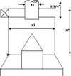Fig. 1 Air cleaner.

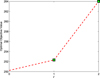Fig. 2 Objective function variation as a function of Γ.

2.1.2 Control of robustness

As was discussed in Section 2.1 that the robust formulation discussed could guarantee a deterministic feasible solution to the robust problem only if Γ ∈ [0, |J_i|]. If more than Γ parameters change than robust formulation is not guaranteed to satisfy all the constraints but it can be shown that actually the optimization problem remains feasible with a high probability level. Specifically, Bertsimas & Sim have shown that even if more than Γ parameters vary, the probability that i^th constraint will be violated is given by: 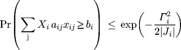$$\text{Pr}(\underset{}{{\displaystyle \sum _{\mathrm{j}}^{}{X}_i}}{a}_{ij}{x}_{ij}\ge b_i)\le \mathrm{e}\mathrm{x}\mathrm{p}(-\frac{{\Gamma }_i^2}{2\left|J_i\right|})$$(7) where exp is the exponential function and .

Using the above approximation, the probability of constraint violation for our problem can be calculated. This gives the decision maker a tradeoff between robustness and cost. It can be seen in Figure 3 that the probability of constraint violation decreases as the degree of conservatism increases.

Fig. 3 Trade-off between robustness and conservatism.

2.2 Non-linear robust optimization

According to [19] There are two forms of perturbations: (1) Implementation errors, which are caused in an imperfect realization of the desired decision variables x, such as those that may occur during the fabrication process; and (2) parameter uncertainties, which are due to modeling errors during the problem definition, such as noise. Most robust optimization formulations, don’t take parameter uncertainties into consideration [1].

Let be the nominal objective of a design problem. The nominal optimization problem ignores uncertainties. Due to factors that are beyond the designer’s control such as manufacturing errors and environmental noises, there can be a lot of uncertainties associated with parameter pp ∈ R^m. Assuming  represents an estimation of the true problem coefficientp. Hence, +Δp can be used instead of p where Δp are the parameter uncertainties. Along with the presence of implementation errors we formulate the robust problem instead of the nominal optimization problem as follows $$\underset{x}{\text{min}}f\left(x,\overline{\mathit{p}}\right)$$

we try to find a design x that minimizes the worst-case cost. $$g\left(x\right):=\underset{\mathrm{\Delta }p\in \mathcal{U}}{\text{max}}f\left(x+\mathrm{\Delta }x,\bar{p}+\mathrm{\Delta }p\right)$$

where △x, Δp is assumed to lie within the uncertainty set u defined as follows $$u=\left\{\mathrm{\Delta }x\in R^n\mathrm{\Delta }p\in R^m\parallel \left[\begin{array}{c}\hfill \mathrm{\Delta }x\hfill \\ \hfill \mathrm{\Delta }p\hfill \end{array}\right]\parallel \le \Gamma \right\}$$(8) where Γ > 0 is the size of perturbation by which the design needs to protected and ||∙||₂ is the l² norm.

For simplicity let’s define 

Having defined the ellipsoidal uncertainty set and the worst-case cost of the objective function, the robust optimization problem which minimizes the worst case cost is given as follows $$\underset{x}{\text{min}}g\left(x\right):=\underset{\mathit{\text{x}}}{\text{min}}\underset{\mathrm{\Delta }z\in \mathcal{U}}{\text{max}}f\left(x+\mathrm{\Delta }x,\overline{p}+\mathrm{\Delta }\text{p}\right)$$

For a constrained problem with ellipsoidal parametric uncertainties such that Γ = 1, the robust formulation would be as follows $$\underset{x}{{\displaystyle \min }}\underset{{||\mathrm{\Delta }z||}_2\le 1}{{\displaystyle \max }}f(x+\mathrm{\Delta }x,\overline{p}+\mathrm{\Delta }p)$$ $$\text{s.t.}\mathrm{.}\underset{{||\mathrm{\Delta }z||}_2\le 1}{\text{max}}h\left(x+\mathrm{\Delta }x,\overline{p}+\mathrm{\Delta }\text{p}\right)\le 0$$(9)

For polyhedral uncertainty set, u is defined as $$\mathit{u}\mathit{=}\{\mathit{\Delta }\mathit{z}\mathit{\in }{\mathit{R}}^{\mathit{n}\mathit{+}\mathit{m}}\mathit{|}\mathit{\sum }\left|\mathrm{\Delta }\mathrm{z}\right|\mathit{\le }\mathit{\Gamma }\}$$(10)

In order to be less restrictive, let’s define a box of uncertainty   with most likely value:  and . Similarly define . Since we are primarily interested in the analysis of parametric data uncertainties, we restrict the ellipsoidal uncertainty set to the parameter uncertainties which are due to modeling errors such as noise in data, which in this case means coefficients of variables. This type of robust optimization formulation requires only modest assumptions about distributions, such as mean and bounded support [20]. Hence making the need for knowledge of underlying probability distributions of stochastic variables unnecessary. $$\underset{\mathit{\text{x}}}{\text{min}}\underset{{||\mathrm{\Delta }z||}_2\le \Gamma }{\text{max}}f\left(x+\mathrm{\Delta }x,\overline{p}+\mathrm{\Delta }\text{p}\right)$$ $$\text{s.t.}\underset{{||\mathrm{\Delta }z||}_2\le \Gamma }{\text{max}}h\left(x+\mathrm{\Delta }x,\overline{p}+\mathrm{\Delta }\text{p}\right)\le 0$$(11) $$-{\sigma }_x\le \Delta x\le {\sigma }_x$$

For linear constraints of the form a′x + b ≤ 0, robustness can be introduced by incorporating robustness level Γ into the constraint as follows $$a^{\prime }x+\Gamma {||a||}_2+b\le 0$$(12)

2.2.1 Example: Robust design of a cantilever beam

The working of the method is demonstrated through an engineering design example from [4]. A cantilever bean in Figure 4 is designed against yielding due to bending stress while the cross-sectional area is desired to be kept as minimum. Five random variables are considered, including two design variables: x = [x₁ , x₂]^T = [b, h]^T and three design parameters p = [p₁, p₂, p₃]^T = [R, Q, L]^T. b and h are the dimensions of the cross-section, L is the length of the beam. Q is the external force and R is the allowable stress of the beam. The objective is to minimize the cross-sectional area of the beam while maximizing its tensile strength. For feasibility the ratio of h/b should also be less than 2. Since the The distributions for the design and parameters are given in Table 1.

The mathematical model is expressed as follows: $$\begin{array}{cc}\hfill \min \hfill & \hfill x_1{x}_2\hfill \end{array}$$ $$\text{s.t.}R-\frac{6QL}{b{h}^2}\ge 0$$ $$2-\frac{x_2}{x_1}\ge 0$$(13)

In this case the parametric uncertainties mean uncertainties in noisy data which manifest themselves in the form of coefficient uncertainties of variables. The robust optimization formulation of the above deterministic problem based on the methodology described above is as follows: $$\begin{array}{ccc}\hfill \underset{x}{\min }\hfill & \hfill \underset{c}{\max }\hfill & \hfill x_1(1+\mathrm{\Delta }{x}_1)x_2(1+\mathrm{\Delta }{x}_2)\hfill \end{array}$$ $$\text{s.t}\mathit{\left(}\mathit{1}\mathit{+}\mathit{\Delta }{\mathit{p}}_{\mathit{1}}\mathit{\right)}\mathit{R}\mathit{-}\frac{\mathrm{6}\mathit{Q}\mathrm{\left(}1+\mathit{\Delta }{\mathit{p}}_{\mathrm{2}}\mathrm{\right)}\mathit{L}\mathrm{\left(}\mathrm{1}\mathrm{+}\mathit{\Delta }{\mathit{p}}_{\mathit{3}}\mathrm{\right)}}{{\mathit{x}}_{\mathrm{1}}\mathrm{\left(}\mathrm{1}\mathit{+}\mathit{\Delta }{\mathit{x}}_{\mathit{1}}\mathrm{\right)}{\mathit{\left(}{\mathit{x}}_{\mathrm{2}}\mathit{\left(}\mathrm{1}\mathrm{+}\mathit{\Delta }{\mathit{x}}_{\mathrm{2}}\mathrm{\right)}\mathrm{\right)}}^{\mathrm{2}}}\ge 0$$ $$2x_1-x_2+\sqrt{5}\mathrm{\Gamma }\ge 0$$ $${\Vert \begin{array}{c}\mathrm{\Delta }x\\ \mathrm{\Delta }p\end{array}\Vert }_2\le \Gamma$$ $$\mathrm{\Delta }x,\mathrm{\Delta }p\mathrm{f}\mathrm{r}\mathrm{e}\mathrm{e}$$ $$x_1,x_2\ge 0$$(14)

Here Δp represents the parametric uncertainties and Δxrepresents the implementation errors.

The result of the optimization are given in Figure 5. Maximum uncertainty was constrained at 10% of the nominal values of the parameters which is the value of standard deviation form the parameters. The flexibility provided by Γ is that it can adjust the design solution based on the level of robustness desired by the designer. When Γ = 0, the robust formulation returns the conventional deterministic solution and when the uncertainty in the design variables and parameters is restricted to 1% then the optimization returns an area that is bigger, as expected, to accommodate all the perturbations in the design space. Compared to other methods discussed in [4], although this method is more conservative but it doesn't have probability of constraint violation as it will always satisfy the strength constraint with a probability of 1.

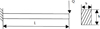Fig. 4 Cantilever beam.

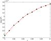Fig. 5 Solution of the beam example as a function of Γ.

3 Robust response surface with uncertain data

Response Surface Methodology (RSM) is an important meta-modeling technique for finding a low order representation of a non trivial process involving multiple design variables. Since the exact relationship between variables and the response is unknown, therefore RSM is used to determine the coefficients for a linear low order polynomial model representation of the response function. A first order response surface model can be represented by the following $$y={\beta }_0+{\beta }_1{x}_1+{\beta }_2{x}_2+\dots +{\beta }_m{x}_m+\epsilon$$

Since a first order function cannot accommodate curvature in the system, and a third and higher order systems become too complicated, therefore in most applications the model is restricted to a second order polynomial as follows [21]. $$y={\beta }_0+\sum _{i=1}^m{\beta }_i{x}_i+\sum _{i=1}^m{\beta }_{ii}{x}_i^2+\sum _{i<j}\sum _{j=2}^m{\beta }_{ij}{x}_i{x}_j+\epsilon$$

For a 2 variable system, this can be simplified to $$y={\beta }_0+{\beta }_1{x}_1+{\beta }_2{x}_2+{\beta }_{11}{x}_1^2+{\beta }_{22}{x}_2^2+{\beta }_{12}{x}_1{x}_2+\epsilon$$(15)

Most of the time we have an over determined system with a set of equations Xβ = Y , where we know the data matrices , . These type of systems are usually solved by minimizing the square of the residuals obtained by the difference between the actual values and the values obtained from the fitted model. This method is known as the method of Least Squares. In the context of our model $$X=\left[\begin{array}{cccccc}\hfill 1\hfill & \hfill x_{11}\hfill & \hfill x_{12}\hfill & \hfill x_{11}^2\hfill & \hfill x_{12}^2\hfill & \hfill x_{11}{x}_{12}\hfill \\ \hfill ⋮\hfill & ⋮& \hfill ⋮\hfill & \hfill ⋮\hfill & \hfill ⋮\hfill & ⋮\\ \hfill 1\hfill & \hfill x_{n1}\hfill & \hfill x_{n2}\hfill & \hfill x_{n1}^2\hfill & \hfill x_{n2}^2\hfill & \hfill x_{n1}\hfill \end{array}\right]$$ $$Y=\left[\begin{array}{c}\hfill y_1\hfill \\ \hfill \begin{array}{l}.\\ .\\ .\end{array}\hfill \\ \hfill y_n\hfill \end{array}\right],\beta =\left[\begin{array}{c}\hfill {\beta }_0\hfill \\ \hfill \begin{array}{l}.\\ .\\ .\end{array}\hfill \\ \hfill {\beta }_m\hfill \end{array}\right]$$

The objective is to minimize the squared error between the fitted model and the actual value by using the residual as the objective function $$r={\parallel X\beta -Y\parallel }^2$$(16)

There is an analytical closed form for determining the coefficients β using the method of least squares which is $$\beta ={\left(X^{T}X\right)}^{-1}{X}^{T}Y$$(17)

Assuming we are facing the same type of uncertainties in the data as we assumed in the previous sections which might be because of manufacturing errors or implementation errors and that can perturb either the elements of matrix X or Y or both in which case the β’s are going to become suboptimal. We are going to assume that the coefficients of matrices X and Y are unknown but bounded as before.

We are going to solve this problem using two methods; Robust Least Squares method and Regularization Method.

3.1 Robust Least Square (RLS) method

We employ the method of Robust Least Squares (RLS) [22] to determine the optimal β’s in this case. RLS method assumes that data matrices are subject to deterministic perturbations such that instead of pairs (X, Y ) we have perturbed pair (X + △ X, Y + △ Y ), where △v = [△ X  △ Y ] is an unknown but bounded matrix with, where ρ ≥ 0 is provided. So we minimize the following residual instead of the one in equation (16). $$\varphi (X,Y,\rho )=\underset{x}{\min }\underset{\left|\right|XY|{|}_2\le \rho }{\max }\left|\right|(X+X)\beta -(Y+Y)\left|\right|$$(18)

It can be seen that for ρ = 0, we recover the original least squares problem.

When ρ = 1, the worst-case residual is given by $$\mathrm{r}\left(X,Y,\beta \right)=||X\mathit{\beta }-Y||+\mathrm{v}{||\beta ||}^2+1$$(19)

A unique solution x_RLS fen by $$x_{RLS}=\{\begin{array}{ll}{(\mu I+X^{T}X)}^{-1}\hfill & if\mu =(\lambda -\tau )/\tau >0\hfill \\ X^{!}Y\hfill & \mathrm{e}\mathrm{l}\mathrm{s}\mathrm{e}\hfill \end{array}$$(20) where X^! denotes the Moore-Penrose pseudo inverse of X and λ and τ are the unique optimal points for the following problem. $$\begin{array}{cc}\hfill \min \mathrm{i}\mathrm{m}\mathrm{i}\mathrm{z}\mathrm{e}\hfill & \hfill \lambda \hfill \end{array}$$ $$\text{subject to}\parallel X\beta -Y\parallel \le \lambda -\tau$$ $$\parallel \left[\begin{array}{c}\hfill x\hfill \\ \hfill 1\hfill \end{array}\right]\parallel \le \tau$$(21)

For comparison purposes, the results of this method will be compared with the one proposed by [23] which is based on minimizing the maximum deviation by building a confidence interval B around the coefficient estimates (β). It is assumed that the true β is some element b of B. The method optimizes the following problem $$\underset{x}{\mathrm{\text{min}}}\underset{\beta \in B}{\mathrm{\text{max}}}\left\{f\left(x,b\right)-g\left(b\right)\right\}$$ $$=\underset{x}{\mathrm{\text{min}}}\underset{i}{\mathrm{\text{max}}}\{f(x,b^i)-g(b^i)\}$$(22) where b¹, b², …,b^M are the extreme points of B and and  

3.1.1 Example: Process robustness under uncertain data

To illustrate the working of this method, an example application of robust manufacturing is taken from [22]. In semiconductor manufacturing we would like the oxide thickness on a wafer to be as close as possible to the target mean thickness. Suppose the semiconductor manufacturing plant has two controllable variables x₁ and x₂. Table 2 shows experiment that was performed. The objective is to find operating conditions that give a minimum mean response, while making the variability of the response as small as possible. In the problem, the true function relating performance response y and design variables x₁ and x₂ has been given by the quadratic function $$y=0.5x_1^2-x_1{x}_2+x_2^2-2x_1-6x_2$$(23)

with the constraints as follows $$x_1+x_2\le 6$$ $$x_1\ge 0$$(24) $$x_2\ge 0$$

The optimal solution to this deterministic problem is (2.8, 3.2) for an optimal value of y = −19.6. It is then supposed that the objective function is not known. A design of experiment study is carried out to estimate the objective function using a 2³ orthogonal array experiment with x_1,2 = −1, 0, 1 as shown in Table 2. An error term ε ~ N (0, 1) is added to the objective function equation to introduce random errors. Monte Carlo simulation is used to analyze the performance of different methodologies compared to the RLS method discussed in the previous section.

The Monte Carlo simulation is performed 100 times and the canonical method of least squares is used to estimate the response surface and subsequent optimal values for the problem. The robust optimization method of Xu & Albin is also used to calculate the robust optimal values, the values of which are given in their paper. They are compared with the RLS method given in the previous section for analysis.

Table 3 indicates that the RLS approach achieves better results for mean performance compared to the robust optimization model of [22] for this test problem using 100 Monte Carlo simulation runs. It turns out that the robust approach of Xu & Albin is slightly more conservative than the one given in this paper. Although this result cannot be generalized for high dimensional equations for ρ > 1 where the poly tope B can turn out to be less conservative but more computationally expensive than the RLS approach.

3.2 Regularization method

Regularization methods provide an alternate methodology for managing uncertainty in data matrices X and Y particularly if these matrices are sensitive to errors or are ill conditioned [23]. In order to restrict the perturbation on β to reduce sensitivity, these methods place a bound on the β vector so that we minimize where Ω is some suitable norm. This method is similar to the classical Tikhonov regularization method when where μ > 0 is a regularization parameter that improves the conditioning of the problem thus making it more suitable for a solution. Solution β is found by solving the following problem $$\text{min}{\parallel X\beta -Y\parallel }^2+\mu {\parallel \beta \parallel }^2$$(25)

and is given by $$\beta \left(\mu \right)={\left(\mu I+X^{T}X\right)}^{-1}{X}^{T}Y$$(26)

If we assume that the values of elements in matrices X and Y are not the nominal values on which perturbation occurs in the form of ΔX and ΔY respectively i.e., X and Y themselves comprise of data measures that have measurement errors. In this case it’s going to be hard to estimate a bound ρ on ΔX and ΔY. Reference [23] proposes a Total Least Squares (TLS) methodology for these problems in which case μ = −σ² where σ is the smallest singular value of  . Hence  .

When we apply TLS to the example problem in Section 3.1.1, we get the results as shown in Table 4.

TLS method gives worst values than all the methods considered before but it is to be expected since it does not consider any bound on the perturbation of data.

4 Conclusions

Three new methods for robust optimization methodologies for linear and non-linear problems were discussed and implemented on practical problems. The methods provide advantages associated with including uncertainty in the model as a safeguard against implementation errors and parametric uncertainties. Uncertainties in response surface models were also considered and simulations show significant improvement of the objective and decrease in variability of the response using the proposed method. The results point to a viable methods that can be used for the robust optimization of mechanical and process design problems under restricted but reasonable perturbations.

Acknowledgments

The author would like to thank his advisor Prof. Daniel D. Frey for his help with this paper and for reviewing the draft.

References

All Tables

All Figures

	Fig. 1 Air cleaner.
In the text

	Fig. 2 Objective function variation as a function of Γ.
In the text

	Fig. 3 Trade-off between robustness and conservatism.
In the text

	Fig. 4 Cantilever beam.
In the text

	Fig. 5 Solution of the beam example as a function of Γ.
In the text

References

- S. Sundaresan, K. Ishii, D.R. Houser, A robust optimization procedure with variations on design variables and constraints, Eng. Optim. 24, 101–117 (1995) [CrossRef] [Google Scholar]
- A. Parkinson, C. Sorensen, N. Pourhassan, A general approach for robust optimal design, J. Mech. Des. 115, 74–80 (1993) [CrossRef] [Google Scholar]
- K.H. Lee, G.J. Park, Robust optimization considering tolerances of design variables, Comput. Struct. 79, 77–86 (2001) [CrossRef] [Google Scholar]
- X. Du, W. Chen, Towards a better understanding of modeling feasibility robustness in engineering design, J. Mech. Des. 122, 385–394 (2000) [CrossRef] [Google Scholar]
- D. Ullman, Robust decision-making for engineering design, J. Eng. Des. 12, 3–13 (2001) [CrossRef] [Google Scholar]
- A. Zakarian, J.W. Knight, L. Baghdasaryan, Modelling and analysis of system robustness., J. Eng. Des. 18, 243–263 (2007) [CrossRef] [Google Scholar]
- J. Olvander, Robustness considerations in multi-objective optimal design, J. Mech. Des 16, 511–523 (2005) [Google Scholar]
- J.S. Kang, M.H. Suh, Robust economic optimization of process design under uncertainty, Eng. Optim. 36, 51–75 (2004) [CrossRef] [Google Scholar]
- J.S. Kang, T.Y. Lee, D.Y. Lee, Robust optimization for engineering design, Eng. Optim. 44, 175–194 (2012) [CrossRef] [Google Scholar]
- L. Wang, X. Wang, X. Yong, Hybrid reliability analysis of structures with multi-source uncertainties, Acta Mech. 225, 413–430 (2014) [CrossRef] [Google Scholar]
- L. Wang, X. Wang, R. Wang, X. Chen, Reliability-based design optimization under mixture of random, interval and convex uncertainties, Arch. Appl. Mech. 86, 1341–1367 (2016) [CrossRef] [Google Scholar]
- L. Wang, X. Wang , H. Su, G. Lin, Reliability estimation of fatigue crack growth prediction via limited measured data, Int. J. Mech. Sci. 121, 44–57 (2017) [CrossRef] [Google Scholar]
- W. Chen, M.M. Wiecek, Compromise programming approach to robust design, J. Mech. Des. 121, 179–188 (1999) [CrossRef] [Google Scholar]
- X. Lu, X. Li, Perturbation theory based robust design under model uncertainty, J. Mech. Des. 131, 111006 (2009) [CrossRef] [Google Scholar]
- B. Huang, X. Du, Analytical robustness assessment for robust design, Struct. Multidiscip. Optim. 34, 123–137 (2007) [CrossRef] [Google Scholar]
- A.L. Soyster, Convex programming with set-inclusive constraints and applications to inexact linear programming, Oper. Res. 21, 1154–1157 (1973) [CrossRef] [Google Scholar]
- D. Bertsimas, M. Sim, The price of robustness, Oper. Res. 52, 35–53 (2004) [CrossRef] [MathSciNet] [Google Scholar]
- S. Advani, Linear programming approach to air-Cleaner design, Oper. Res. 22, 295–297 (1974) [CrossRef] [Google Scholar]
- D. Bertsimas, O. Nohadani, Nonconvex robust optimization for problems with constraints, INFORMS J. Comput. 22, 22–58 (2009) [Google Scholar]
- X. Chen, M. Sim, P. Sun, A robust optimization perspective on stochastic programming, Oper. Res. 55, 1058 (2007) [CrossRef] [Google Scholar]
- D.C. Montgomery, Introduction to Statistical Quality Control, edited by N.J. Hoboken (John Wiley & Sons Inc., New York, 2009) [Google Scholar]
- D. Xu, S.L. Albin, Robust optimization of experimentally derived objective functions, IIE Trans. 35, 793–802 (2003) [CrossRef] [Google Scholar]
- L.El. Ghaoui, H. Laurent, Robust solutions to least-squares problems with uncertain data, SIAM J. Matrix Anal. Appl. 18, 1035 (1997) [CrossRef] [Google Scholar]
Cite this article as: Hassan J. Bukhari, Robust design optimization using the price of robustness, robust least squares and regularization methods, Int. J. Simul. Multidisci. Des. Optim. 8, A13 (2017)